Price Action Analysis Toolkit Development (Part 36): Unlocking Direct Python Access to MetaTrader 5 Market Streams

Contents

• Introduction
• System Architecture Overview
• Detailed Examination of the Python Backend
• Exploring the MQL5 EA Client Architecture
• Evaluation & Performance Outcomes
• Conclusion

Introduction

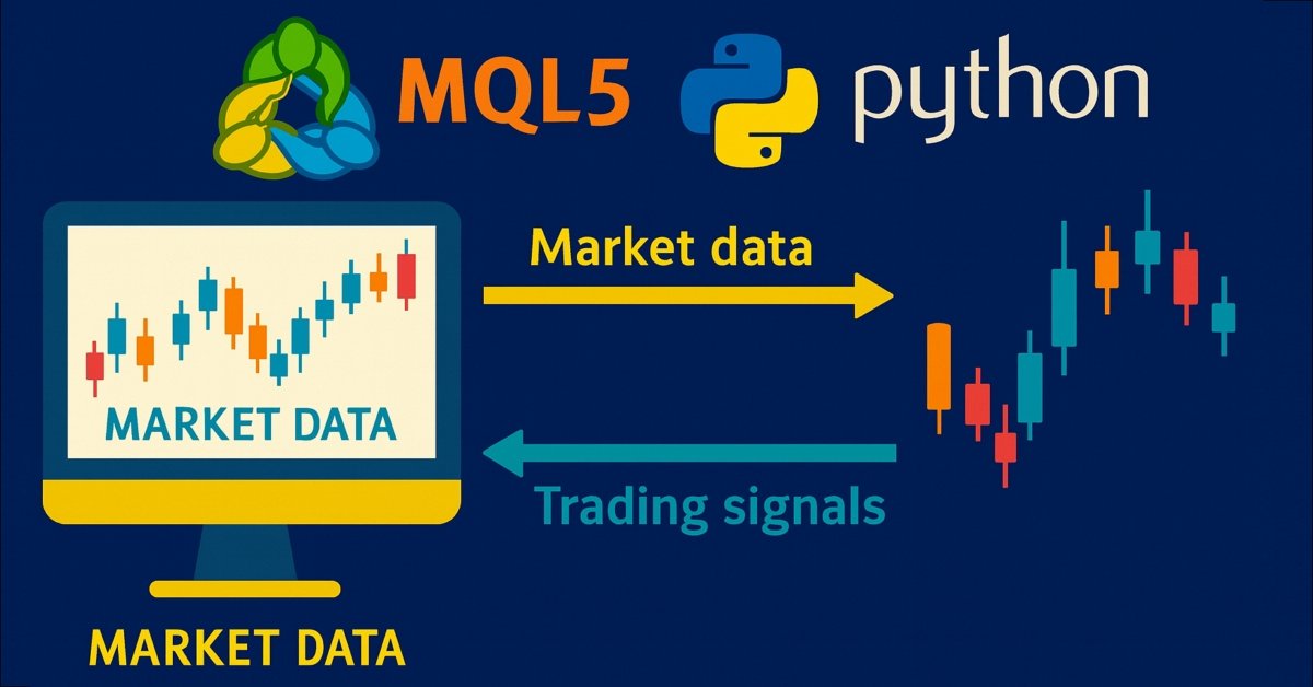
Our previous article demonstrated how a straightforward MQL5 script could transfer historical bars into Python, engineer features, train a machine learning model, and then send signals back to MetaTrader for execution—eliminating manual CSV exports, Excel-based analysis, and version control issues. Traders gained an end-to-end pipeline that transformed raw minute-bar data into statistically driven entry points, complete with dynamically calculated stop-loss (SL) and take-profit (TP) levels.

This system addressed three major pain points in algorithmic trading:

1. Data Fragmentation: No more copying and pasting CSV files or dealing with complex spreadsheet formulas—your MetaTrader 5 chart communicates directly with Python.
2. Delayed Insights: Automating feature engineering and model inference enabled real-time signals, shifting from reactionary to proactive trading based on live data.
3. Inconsistent Risk Management: Incorporating ATR-based SL/TP into both backtests and live trading ensured all trades followed volatility-adjusted rules, preserving your edge.

However, relying on an Expert Advisor (EA) to feed data into Python can introduce latency and complexity. The new release leverages Python’s capability to act as an MetaTrader 5 client—using the MetaTrader 5 library to fetch and update data directly. This approach eliminates the wait for an EA timer; Python can ingest data on demand, write efficiently to a Parquet store, and run heavy computations asynchronously.

Building on this foundation, our enhanced Python–MQL5 hybrid tool offers even greater capabilities:

• Python Side: Real-time MetaTrader 5 data ingestion via the native library, advanced feature engineering (e.g., spike z-scores, MACD differences, ATR bands, Prophet trend deltas), and a TimeSeries-aware Gradient Boosting pipeline that retrains on rolling windows—all exposed through a lightweight Flask API.
• MQL5 Side: A robust REST-polling EA with retry logic, an on-chart dashboard displaying signals, confidence levels, and connection status, arrow markers for entries and exits, and optional automated order execution under strict risk management rules.

While our first article provided a proof-of-concept, this production-grade framework significantly reduces setup time, accelerates feedback loops, and empowers you to trade with data-backed confidence and precision. Let’s dive in

System Architecture Overview

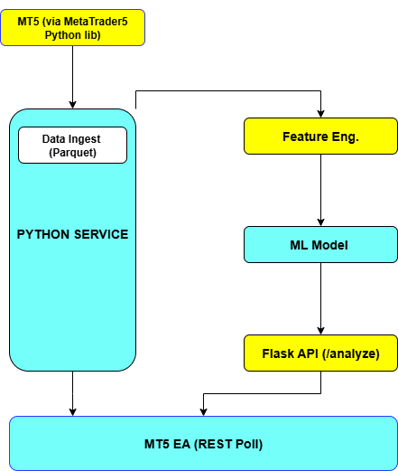
Below is a high-level flow of how data and signals traverse between MetaTrader 5 and your Python service, followed by the core responsibilities of each component:

MetaTrader 5 Terminal

The MetaTrader 5 terminal serves as the primary market interface and charting platform. It hosts the live and historical price bars for your chosen symbol and provides the execution environment for the Expert Advisor (EA). Through its built-in WebRequest() functionality, the EA periodically gathers the latest bar data and displays incoming signals, SL/TP lines, and entry/exit arrows directly on your chart. The MetaTrader 5 Terminal is responsible for order placement (when enabled), local object management (panels, arrows, labels), and user-facing visualization of the system’s outputs.

Python Data Feed

Rather than relying on an EA to push bar data, the Python Data Feed component uses the official MetaTrader 5 Python library to pull both historical and real-time minute-bar OHLC data on demand. It bootstraps a compressed Parquet datastore to persist past days of price action and then appends new bars as they arrive. This setup eliminates dependencies on timer intervals in MQL5 and ensures that the Python service always has immediate, random-access to the full price history needed for both backtests and live inference.

Feature Engineering

Once raw bars are available in memory or on disk, the Feature Engineering layer transforms them into statistically meaningful inputs for machine learning. It computes normalized spike z-scores, the MACD histogram difference, 14-period RSI values, 14-period ATR for volatility, and dynamic EMA-based envelope bands. Additionally, it leverages Facebook’s Prophet library to estimate a minute-level trend delta, capturing mean-reversion vs. trending bias. This automated pipeline guarantees that live and historical data undergo identical processing, preserving model fidelity.

ML Model

At the heart of the system lies a Gradient Boosting classifier wrapped in a scikit-learn Pipeline with standard scaling. The model is trained on rolling windows of past bars, using TimeSeriesSplit to avoid look-ahead bias and RandomizedSearchCV to optimize hyperparameters. Labels are generated by looking ten minutes forward in price and categorizing moves into buy, sell, or wait classes based on a configurable threshold. The trained estimator is serialized to model.pkl, ensuring low latency loading and inference in both backtests and live runs.

Flask API

The Flask API serves as the bridge between Python’s data-science ecosystem and the MQL5 EA. It exposes a single/analyze endpoint that accepts a JSON payload of recent closes and timestamps, applies the feature pipeline and loaded model to compute class probabilities, and returns a concise JSON response containing signal, sl, tp, and conf (confidence). This lightweight REST interface can be containerized or deployed on any server, decoupling your Python compute resources from MetaTrader’s runtime environment and simplifying scalability.

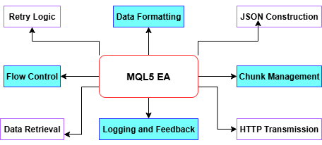
MQL5 Expert Advisor

On the client side, the MQL5 EA focuses exclusively on user interaction and trade execution. It periodically polls the Flask API, parses incoming JSON, logs each signal to both the Experts tab and a local CSV file, and updates an on-chart dashboard showing the current signal, confidence level, connection status, and timestamp. When a valid buy, sell, or close signal arrives, the EA draws arrows and SL/TP lines and—if EnableTrading is true—places or closes orders via the CTrade class. By offloading all data science to Python, the EA remains lean, responsive, and easy to maintain.

Detailed Examination of the Python Backend

At the foundation of our backend lies a robust data‐ingestion pipeline that leverages the official MetaTrader 5 Python package. On first run, the service “bootstraps” by fetching the last days of minute-bar OHLC data and writing it into a compressed Parquet file. Parquet’s columnar format and Zstandard compression yield blazing-fast reads for time-series slices, while keeping disk usage minimal. Thereafter, a simple incremental update appends only newly formed bars—avoiding redundant downloads and ensuring that both live inference and backtests operate on an up-to-date, single source of truth.

import datetime as dt
import pandas as pd
import MetaTrader5 as mt5
from pathlib import Path

PARQUET_FILE = "hist.parquet.zst"
DAYS_TO_PULL = 60
UTC = dt.timezone.utc

def bootstrap():
    """Fetch last DAYS_TO_PULL days of M1 bars and write to Parquet."""
    now = dt.datetime.utcnow()
    start = now - dt.timedelta(days=DAYS_TO_PULL)
    mt5.initialize()
    mt5.symbol_select("Boom 300 Index", True)
    bars = mt5.copy_rates_range("Boom 300 Index", mt5.TIMEFRAME_M1,
                                start.replace(tzinfo=UTC),
                                now.replace(tzinfo=UTC))
    df = pd.DataFrame(bars)
    df['time'] = pd.to_datetime(df['time'], unit='s')
    df.set_index('time').to_parquet(PARQUET_FILE, compression='zstd')

def append_new_bars():
    """Append only the newest bars since last timestamp."""
    df = pd.read_parquet(PARQUET_FILE)
    last = df.index[-1]
    now = dt.datetime.utcnow()
    new = mt5.copy_rates_range("Boom 300 Index", mt5.TIMEFRAME_M1,
                               last.replace(tzinfo=UTC) + dt.timedelta(minutes=1),
                               now.replace(tzinfo=UTC))
    if new:
        new_df = pd.DataFrame(new)
        new_df['time'] = pd.to_datetime(new_df['time'], unit='s')
        merged = pd.concat([df, new_df.set_index('time')])
        merged[~merged.index.duplicated()].to_parquet(PARQUET_FILE,
                                                      compression='zstd')

With raw bars in place, our pipeline computes a suite of features designed to capture momentum, volatility, and extreme moves. We normalize the first difference of price into a "z-spike" score by dividing by its 20-bar rolling standard deviation, isolating sudden price surges. MACD histogram difference and 14-period RSI quantify trend and overbought/oversold conditions, respectively, while 14-period ATR measures current volatility. A 20-period EMA defines envelope bands (EMA×0.997 and EMA×1.003) that adapt to shifting regimes. Finally, Facebook’s Prophet library ingests the entire close-price series to forecast a minute-level trend delta—capturing more nuanced, time-dependent seasonality and drift.

import numpy as np
import pandas as pd
import ta
from prophet import Prophet

def engineer(df: pd.DataFrame) -> pd.DataFrame:
    df = df.copy()
    # z-spike (20-bar rolling std)
    df['r'] = df['close'].diff()
    df['z_spike'] = df['r'] / (df['r'].rolling(20).std() + 1e-9)

    # MACD histogram diff, RSI, ATR
    df['macd'] = ta.trend.macd_diff(df['close'])
    df['rsi']  = ta.momentum.rsi(df['close'], window=14)
    df['atr']  = ta.volatility.average_true_range(df['high'],
                                                  df['low'],
                                                  df['close'],
                                                  window=14)

    # EMA envelopes
    ema = df['close'].ewm(span=20).mean()
    df['env_low'] = ema * 0.997
    df['env_up']  = ema * 1.003

    # Prophet trend delta (minute-level)
    if len(df) > 200:
        m = Prophet(daily_seasonality=False, weekly_seasonality=False)
        m.fit(pd.DataFrame({'ds': df.index, 'y': df['close']}))
        df['delta'] = m.predict(m.make_future_dataframe(periods=0,
                                                        freq='min'))['yhat'] - df['close']
    else:
        df['delta'] = 0.0

    return df.dropna()

We frame prediction as a three-class classification: “BUY” if price moves up by more than a threshold over the next 10 minutes, “SELL” if it falls by more than that threshold, and “WAIT” otherwise. Once labels are assigned, features and labels are split into rolling time windows for training. A scikit-learn Pipeline first standardizes each feature, then fits a GradientBoostingClassifier. Hyperparameters (learning rate, tree count, max depth) are optimized via RandomizedSearchCV under a TimeSeriesSplit cross-validation scheme, ensuring no look-ahead leakage. The best model is serialized to model.pkl, ready for immediate, low-latency inference.

import numpy as np
import joblib
from sklearn.pipeline import Pipeline
from sklearn.preprocessing import StandardScaler
from sklearn.ensemble import GradientBoostingClassifier
from sklearn.model_selection import TimeSeriesSplit, RandomizedSearchCV

LOOKAHEAD_MIN   = 10
LABEL_THRESHOLD = 0.0015
FEATS = ['z_spike','macd','rsi','atr','env_low','env_up','delta']

def label_and_train(df: pd.DataFrame):
    # Look-ahead return
    chg = (df['close'].shift(-LOOKAHEAD_MIN) - df['close']) / df['close']
    df['label'] = np.where(chg > LABEL_THRESHOLD, 1,
                   np.where(chg < -LABEL_THRESHOLD, 2, 0))

    X = df[FEATS].dropna()
    y = df.loc[X.index, 'label']

    pipe = Pipeline([
        ('scaler', StandardScaler()),
        ('gb', GradientBoostingClassifier(random_state=42))
    ])
    param_dist = {
        'gb__learning_rate': [0.01, 0.05, 0.1],
        'gb__n_estimators': [300, 500, 700],
        'gb__max_depth': [2, 3, 4]
    }
    cv = TimeSeriesSplit(n_splits=5)
    rs = RandomizedSearchCV(pipe, param_dist, n_iter=12,
                            cv=cv, scoring='roc_auc_ovr',
                            n_jobs=-1, random_state=42)
    rs.fit(X, y)
    joblib.dump(rs.best_estimator_, 'model.pkl')

To bridge Python and MetaTrader, we expose a single Flask endpoint, /analyze. Clients send a JSON payload containing symbol, an array of close prices, and corresponding UNIX timestamps. The endpoint replays our feature pipeline on that payload, loads the pre-trained model, computes class probabilities, determines the highest-confidence signal, and dynamically derives stop-loss and take-profit levels from the ATR feature. The response is a compact JSON object:

from flask import Flask, request, jsonify
import joblib
import pandas as pd

app = Flask(__name__)
model = joblib.load('model.pkl')

@app.route('/analyze', methods=['POST'])
def analyze():
    payload = request.get_json(force=True)
    closes = payload['prices']
    times  = pd.to_datetime(payload['timestamps'], unit='s')
    df = pd.DataFrame({'close': closes}, index=times)
    # duplicate open/high/low for completeness
    df[['open','high','low']] = df[['close']]

    feat = engineer(df).iloc[-1:]
    probs = model.predict_proba(feat[FEATS])[0]
    p_buy, p_sell = probs[1], probs[2]
    signal = ('BUY' if p_buy > 0.55 else
              'SELL' if p_sell > 0.55 else 'WAIT')
    atr = feat['atr']
    entry = feat['close']
    sl = entry - atr if signal=='BUY' else entry + atr
    tp = entry + 2*atr if signal=='BUY' else entry - 2*atr

    return jsonify(signal=signal,
                   sl=round(sl,5),
                   tp=round(tp,5),
                   conf=round(max(p_buy,p_sell),2))

if __name__ == '__main__':
    app.run(port=5000)

Exploring the MQL5 EA Client Architecture

The EA’s core loop lives in either a timer event (OnTimer) or a new-bar check, where it invokes WebRequest() to send and receive HTTP messages. First, it gathers the most recent N bars via CopyRates, converts the MqlRates array into a UTF-8 JSON payload containing symbol and close-price sequence, and sets the required HTTP headers. If WebRequest() fails (returns ≤0), the EA captures GetLastError(), increments a retry counter, logs the error, and postpones further requests until either retries are exhausted or the next timer tick. Successful responses (status ≥200) reset the retry count and update lastStatus. This pattern ensures robust, asynchronous signaling without blocking the chart thread or crashing on transient network hiccups.

// In OnTimer() or OnNewBar():
MqlRates rates[];
// Copy the last N bars into `rates`
if(CopyRates(_Symbol, _Period, 0, InpBufferBars, rates) != InpBufferBars)
    return;
ArraySetAsSeries(rates, true);

// Build payload
string payload = "{";
payload += StringFormat("\"symbol\":\"%s\",", _Symbol);
payload += "\"prices\":[";
for(int i=0; i<InpBufferBars; i++)
  {
    payload += DoubleToString(rates[i].close, _digits);
    if(i < InpBufferBars-1) payload += ",";
  }
payload += "]}";

// Send request
string headers = "Content-Type: application/json\r\nAccept: application/json\r\n\r\n";
char  req[], resp[];
int   len = StringToCharArray(payload, req, 0, WHOLE_ARRAY, CP_UTF8);
ArrayResize(req, len);
ArrayResize(resp, 8192);

int status = WebRequest("POST", InpServerURL, headers, "", InpTimeoutMs,
                        req, len, resp, headers);
if(status <= 0)
{
  int err = GetLastError();
  PrintFormat("WebRequest error %d (attempt %d/%d)", err, retryCount+1, MaxRetry);
  ResetLastError();
  retryCount = (retryCount+1) % MaxRetry;
  lastStatus = StringFormat("Err%d", err);
  return;
}
retryCount = 0;
lastStatus = StringFormat("HTTP %d", status);

Once a valid JSON reply is parsed into a signal, sl, and tp, the EA updates its on-chart dashboard and draws any new arrows or lines. The dashboard is a single OBJ_RECTANGLE_LABEL with four text labels showing symbol, current signal, HTTP status, and timestamp. For trades, it deletes any existing prefixed objects before creating a fresh arrow (OBJ_ARROW) at the current price, using distinct arrow codes and colors for buy (green up), sell (red down), or close (orange). Horizontal lines (OBJ_HLINE) mark Stop-Loss and Take-Profit levels color-coded red and green respectively. By name spacing each object with a chart-unique prefix and cleaning them up on signal changes or deinitialization, your chart remains crisp and uncluttered.

// Panel (rectangle + labels)
void DrawPanel()
{
  const string pid = "SigPanel";
  if(ObjectFind(0, pid) < 0)
    ObjectCreate(0, pid, OBJ_RECTANGLE_LABEL, 0, 0, 0);

  ObjectSetInteger(0, pid, OBJPROP_CORNER, CORNER_LEFT_UPPER);
  ObjectSetInteger(0, pid, OBJPROP_XDISTANCE, PanelX);
  ObjectSetInteger(0, pid, OBJPROP_YDISTANCE, PanelY);
  ObjectSetInteger(0, pid, OBJPROP_XSIZE, PanelW);
  ObjectSetInteger(0, pid, OBJPROP_YSIZE, PanelH);
  ObjectSetInteger(0, pid, OBJPROP_BACK, true);
  ObjectSetInteger(0, pid, OBJPROP_BGCOLOR, PanelBG);
  ObjectSetInteger(0, pid, OBJPROP_COLOR, PanelBorder);

  string lines[4] = {
    StringFormat("Symbol : %s", _Symbol),
    StringFormat("Signal : %s", lastSignal),
    StringFormat("Status : %s", lastStatus),
    StringFormat("Time   : %s", TimeToString(TimeLocal(), TIME_MINUTES))
  };

  for(int i=0; i<4; i++)
  {
    string lbl = pid + "_L" + IntegerToString(i);
    if(ObjectFind(0, lbl) < 0)
      ObjectCreate(0, lbl, OBJ_LABEL, 0, 0, 0);
    ObjectSetInteger(0, lbl, OBJPROP_CORNER, CORNER_LEFT_UPPER);
    ObjectSetInteger(0, lbl, OBJPROP_XDISTANCE, PanelX + 6);
    ObjectSetInteger(0, lbl, OBJPROP_YDISTANCE, PanelY + 4 + i*(TxtSize+2));
    ObjectSetString(0, lbl, OBJPROP_TEXT, lines[i]);
    ObjectSetInteger(0, lbl, OBJPROP_FONTSIZE, TxtSize);
    ObjectSetInteger(0, lbl, OBJPROP_COLOR, TxtColor);
  }
}

// Arrows & SL/TP lines
void ActOnSignal(ESignal code, double sl, double tp)
{
  // remove old arrows/lines
  for(int i=ObjectsTotal(0)-1; i>=0; i--)
    if(StringFind(ObjectName(0,i), objPrefix) == 0)
      ObjectDelete(0, ObjectName(0,i));

  // arrow
  int    arrCode = (code==SIG_BUY ? 233 : code==SIG_SELL ? 234 : 158);
  color  clr     = (code==SIG_BUY ? clrLime : code==SIG_SELL ? clrRed : clrOrange);
  string name    = objPrefix + "Arr_" + TimeToString(TimeCurrent(), TIME_SECONDS);
  ObjectCreate(0, name, OBJ_ARROW, 0, TimeCurrent(), SymbolInfoDouble(_Symbol, SYMBOL_BID));
  ObjectSetInteger(0, name, OBJPROP_ARROWCODE, arrCode);
  ObjectSetInteger(0, name, OBJPROP_COLOR, clr);

  // SL line
  if(sl > 0)
  {
    string sln = objPrefix + "SL_" + name;
    ObjectCreate(0, sln, OBJ_HLINE, 0, 0, sl);
    ObjectSetInteger(0, sln, OBJPROP_COLOR, clrRed);
  }

  // TP line
  if(tp > 0)
  {
    string tpn = objPrefix + "TP_" + name;
    ObjectCreate(0, tpn, OBJ_HLINE, 0, 0, tp);
    ObjectSetInteger(0, tpn, OBJPROP_COLOR, clrLime);
  }
}

Actual order placement is gated behind an EnableTrading flag, so you can switch effortlessly between visual-only and live-execution modes. Before any market order, the EA checks PositionSelect(_Symbol) to avoid duplicate positions. For a BUY signal, it invokes CTrade.Buy() with FixedLots, SL, and TP; for SELL, CTrade.Sell(); and for a CLOSE signal, CTrade.PositionClose(). Slippage tolerance (SlippagePoints) is applied on exits. This minimal, stateful logic ensures you never accidentally enter the same side twice and that all orders respect your predefined risk parameters.

void ExecuteTrade(ESignal code, double sl, double tp)
{
  if(!EnableTrading) return;

  bool hasPosition = PositionSelect(_Symbol);
  if(code == SIG_BUY && !hasPosition)
    trade.Buy(FixedLots, _Symbol, 0, sl, tp);
  else if(code == SIG_SELL && !hasPosition)
    trade.Sell(FixedLots, _Symbol, 0, sl, tp);
  else if(code == SIG_CLOSE && hasPosition)
    trade.PositionClose(_Symbol, SlippagePoints);
}

Installation and Configuration

Before you can begin generating live signals, you’ll need to prepare both your Python environment and your MetaTrader 5 platform. Start by installing Python 3.8 or newer on the same machine where your MetaTrader 5 terminal runs. Create and activate a virtual environment (python -m venv venv then on Windows venv\Scripts\activate, or on macOS/Linux source venv/bin/activate) and install all dependencies with:

pip install MetaTrader 5 pandas numpy ta prophet scikit-learn flask loguru joblib

Next, configure your Windows firewall to allow outbound HTTP requests for both python.exe and terminal64.exe. If you plan to deploy over HTTPS in production, install your SSL certificate in the Trusted Root certificate store so MetaTrader 5 will accept secure connections.

On the MetaTrader 5 side, open

Tools → Options → Expert Advisors, enable DLL imports, and add your local API host

For example, (http://127.0.0.1:5000) to the “Allow WebRequest for listed URL” box. This whitelist step is crucial—without it, MetaTrader 5 will silently drop all POST payloads.

In your project folder, copy the Python service script (e.g. market_ai_engine.py) into a working directory of your choice. Edit the top of the script to set your trading symbol (MAIN_SYMBOL), your MetaTrader 5 login credentials (LOGIN_ID, PASSWORD, SERVER), and file paths (PARQUET_FILE, MODEL_FILE). If you prefer a non-default port for the Flask server, you can pass it via --port when you launch the service.
To deploy the Expert Advisor, place the compiled EA.ex5 (or its .mq5 source file) into your MetaTrader 5 installation under MQL5 → Experts.

Restart MetaTrader 5 or refresh the Navigator so that the EA appears in your list. Drag it onto an M1 chart of the same symbol you configured in Python. In the EA’s inputs, point InpServerURL to http://127.0.0.1:5000/analyze, set InpBufferBars (e.g. 60),InpPollInterval (e.g. 60 seconds), and InpTimeoutMs (e.g. 5000 ms). Keep EnableTrading off initially so you can verify signals without executing real orders.

Finally, launch your Python backend in the following sequence:

1. python market_ai_engine.py bootstrap

2. python market_ai_engine.py collect 

3. python market_ai_engine.py train

4. python market_ai_engine.py serve --port 5000

With the Flask server running and AutoTrading enabled in MetaTrader, the EA will begin polling for live signals, drawing arrows and SL/TP lines on your chart, and—once you’re confident, placing trades under your predefined risk rules.

Troubleshooting

If the EA shows no data or always returns “WAIT,” confirm that your API URL is whitelisted in MetaTrader 5’s Expert Advisor settings. For mixed HTTP/HTTPS environments, use plain HTTP (127.0.0.1) for local testing and switch to HTTPS with a trusted certificate for production. Ensure both your server and MetaTrader 5 terminal clocks are synchronized (either both in UTC or the same local time zone) to avoid misaligned bar requests. Finally, verify AutoTrading is turned on and that no global permissions or other EAs are blocking your expert.

Evaluation & Performance Outcomes

To begin working with the hybrid Python–MQL5 machine learning system, the first step is to bootstrap historical data using the command

python market_ai_engine.py bootstrap

This initializes a local dataset by downloading the last 60 days of M1 (1-minute) bars directly from MetaTrader 5 using the native Python MetaTrader 5 library. The data is stored in a compressed Parquet file (hist.parquet.zst), which provides fast disk access and efficient storage. This step needs to be performed only once—unless you want to reset the historical data entirely.

C:\Users\hp\Desktop\Intrusion Trader>python market_ai_engine.py bootstrap
2025-08-04 23:39:23 | INFO | Bootstrapped historical data: 86394 rows

Once bootstrapped, continuous updates can be maintained by running

python market_ai_engine.py collect

This ensures the dataset remains current in real time. While this collector can run in the background, it is only essential if you want a continuously updated stream without needing to re-bootstrap before each training.

C:\Users\hp\Desktop\Intrusion Trader>python market_ai_engine.py collect
2025-08-04 23:41:01 | INFO | Appended 2 new bars
2025-08-04 23:42:01 | INFO | Appended 1 new bars
2025-08-04 23:43:01 | INFO | Appended 1 new bars

With an up-to-date dataset in place, the next step is model training. 

python market_ai_engine.py train

It triggers the full machine learning pipeline. The script reads the Parquet file, applies feature engineering techniques (such as spike detection, MACD differentials, RSI, ATR bands, EMA envelopes, and Prophet-based trends), and then uses a GradientBoostingClassifier wrapped with RandomizedSearchCV to train a predictive model on a rolling window of recent data. The result is a serialized model saved as model.pkl, ready for inference.

C:\Users\hp\Desktop\Intrusion Trader>python market_ai_engine.py train
23:48:44 - cmdstanpy - INFO - Chain [1] start processing
23:51:24 - cmdstanpy - INFO - Chain [1] done processing
2025-08-05 02:59:08 | INFO | Model training complete

To evaluate how well the model might perform in real trading, you can run a backtest using the command

python market_ai_engine.py backtest --days 30

This simulates signal generation and trade outcomes over the past 30 days, calculating metrics such as signal accuracy, win/loss ratios, and overall profitability. Results are saved in a CSV file for easy analysis, offering insights into whether the system’s strategy aligns with your expectations.

C:\Users\hp\Desktop\Intrusion Trader>python market_ai_engine.py backtest --days 30
06:57:33 - cmdstanpy - INFO - Chain [1] start processing
06:58:30 - cmdstanpy - INFO - Chain [1] done processing
2025-08-05 06:59:20 | INFO | Backtest results saved to backtest_results_30d.csv

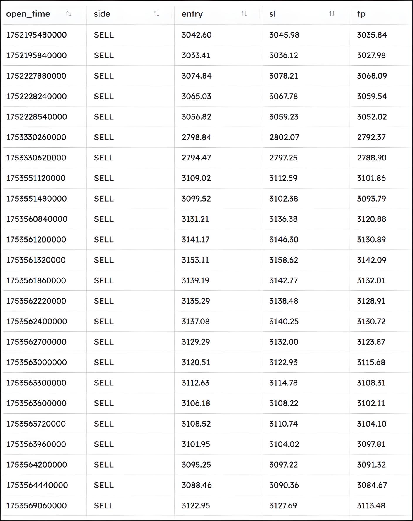
Backtest Results

Below are selected metrics and trade details extracted from the 30-day backtest results:

Cumulative Equity Over Time Graph

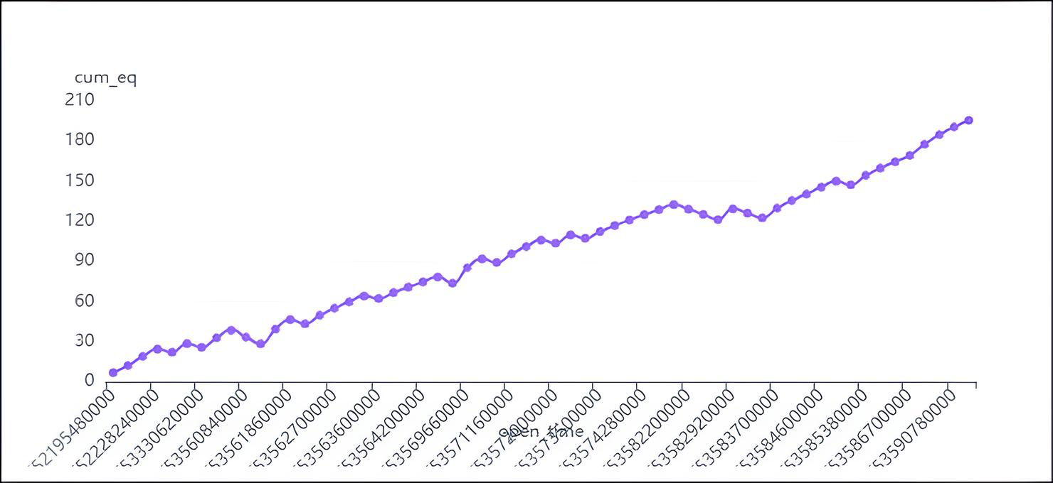
Here's a summary of the key metrics:

*   **Average Entry Price:** 3099.85
*   **Average Exit Price:** 3096.53
*   **Average PNL (Profit and Loss):** 3.32
*   **Total PNL:** 195.69
*   **Average Cumulative Equity:** 96.34
*   **First Trade Time:** 2025-07-11 14:18:00
*   **Last Trade Time:** 2025-07-27 02:00:00

Winrate:

win_rate
72.88135528564453
The win rate is 72.88%. This means that approximately 73% of the trades resulted in a profit.

After the model is trained and validated, you can launch the live inference server with

python market_ai_engine.py serve --port 5000

This command starts a lightweight Flask API that listens for incoming requests from your MQL5 EA. When the EA polls the /analyze endpoint, the server instantly fetches the most recent bar, engineers its features, runs the model, and returns a prediction with corresponding SL, TP, and confidence values in JSON format. This server acts as the live bridge between your chart and the AI engine.

2025-08-05 12:41:53 | INFO | analyze: signal=%s, sl=%.5f, tp=%.5f
127.0.0.1 - - [05/Aug/2025 12:41:53] "POST /analyze HTTP/1.1" 200 -

On the MetaTrader side, the EA must be properly configured to poll the Python server. Within the EA's inputs, the server URL (e.g., http://127.0.0.1:5000/analyze) should be defined, and the EA must be attached to the same symbol and timeframe that the model was trained on—typically M1. Once running, the EA will fetch signals periodically, render them as arrows on the chart, and optionally execute trades based on strict risk rules.

2025.08.05 12:41:53.532 trained model (1) (Boom 300 Index,M1)   >>> JSON: {"symbol":"Boom 300 Index","prices":[2701.855,2703.124,
2704.408,2705.493,2705.963,2696.806,2698.278,2699.877,2701.464,2702.788,2691.762,2693.046,2694.263,2695.587,2696.863,2698.
179,2699.775,2701.328,2702.888,2698.471,2699.887,2695.534,2696.952,2698.426,2699.756,2699.552,2700.954,2702.131,2703.571,
2699.549,2700.868,2702.567,2703.798,2705.067,2706.874,2698.084,2699.538,2700.856,2702.227,2703.692,2705.102,2706.188,2707.609,2709.001,
2710.335,2711.716,2712.919,2712.028,2713.529,2715.052,2716.578,2717.
2025.08.05 12:41:53.943 trained model (1) (Boom 300 Index,M1)   <<< HTTP 200 hdr:
2025.08.05 12:41:53.943 trained model (1) (Boom 300 Index,M1)   {"conf":0.43,"signal":"WAIT","sl":2725.04317,"tp":2720.18266}
2025.08.05 12:41:53.943 trained model (1) (Boom 300 Index,M1)   [2025.08.05 12:41:53] Signal → WAIT | SL=2725.04317 | TP=2720.18266 | Conf=0.43

Conclusion

In this article, we’ve built an MQL5 Expert Advisor that leans on Python’s data-science strengths. Here’s what you now have:

• Data plumbing: your EA pulls minute-bars from MetaTrader 5 and writes them to Parquet.
• Feature engineering: it computes spike-z, MACD, RSI, ATR, envelope bands and even Prophet-based trend deltas.
• Modeling & serving: you train a time-aware Gradient-Boosting model and expose predictions via Flask.
• On-chart action: MQL5 consumes those signals to draw arrows, SL/TP lines—and can place trades automatically.

Along the way you handled real-world quirks, from extra-data JSON parsing in Flask to throttling HTTP calls in your EA and saw how splitting concerns keeps everything maintainable and extensible.
You can try swapping in another algorithm (XGBoost, LSTM, you name it), sharpen your risk-management rules, or containerize the Python service with Docker for cleaner deployments. With this foundation, you’re all set to refine your backtests and push your automated strategies even further.

Chart Projector	Analytical Comment	Analytics Master	Analytics Forecaster	Volatility Navigator	Mean Reversion Signal Reaper
Signal Pulse	Metrics Board	External Flow	VWAP	Heikin Ashi	FibVWAP
RSI DIVERGENCE	Parabolic Stop and Reverse (PSAR)	Quarters Drawer Script	Intrusion Detector	TrendLoom Tool	Quarters Board
ZigZag Analyzer	Correlation Pathfinder	Market Structure Flip Detector Tool	Correlation Dashboard	Currency Strength Meter	PAQ Analysis Tool
Dual EMA Fractal Breaker	Pin bar, Engulfing and RSI divergence	Liquidity Sweep	Opening Range Breakout Tool	Boom and Crash Interceptor	CCI Zer-Line EA
Candlestick Recognition	Candlestick Detection using TA-Lib	Candle Range Tool	MetaTrader 5 Data Ingestor	Model Training and Deployment	Use of Python Lib