MQL5 Wizard Techniques you should know (Part 80): Using Patterns of Ichimoku and the ADX-Wilder with TD3 Reinforcement Learning

Introduction

The terrain of trading with algorithms has evolved steadily from the static indicator based strategies to more dynamic methods that adapt to changing market conditions. One of the most promising methods at this frontier is Reinforcement Learning. Recall, we have already examined implementations of this as well as Inference Learning in prototype wizard assembled Expert Advisors. Unlike classical machine learning methods, that do predictions or classifications, Reinforcement Learning (RL) enables an agent to learn by interacting with its environment. When trading, this implies observing price features continuously, choosing actions such as buy, sell, or hold, and receiving rewards in the form of profit or loss.

In the family of RL algorithms, Twin Delayed Deep Deterministic Policy Gradient (TD3) is emerging, in some circles, as a solid candidate for financial applications. TD3 is designed for continuous action spaces, making it particularly well-suited to trading problems where position sizing and timing are not binary but require fine-grained control. If we compare it to its predecessor, DDPG, TD3 brings in crucial stability improvements such as using more than one critic, adding noise smoothing to the target actions and also delaying policy updates to prevent overfitting to transient fluctuations. 

Our core aim with this article, as always, is to demonstrate how TD3 models, when trained in python, can be merged into MQL5’s Expert Advisor framework, for prototyping. Specifically, we aim to demonstrate how a TD3 actor network that gets exported to the ONNX format can be wrapped and consumed inside a custom signal class. As always, these signal classes then get assembled into a trading robot using the MQL5 Wizard.

To anchor this discussion with some more ‘practicality’, the article will conclude with a review of some forward tests performed in MetaTrader’s Strategy Tester. Three reports are analyzed each covering the 3 signal patterns we had chosen for further study in the ‘Part-74’ article. These were the signal patterns 0, 1, and 5.

Background on RL in Trading

RL is built on a simple yet potent cycle - an agent interacts with an environment, takes actions, and learns from the rewards it receives. To appreciate how we utilize this in trading, it may help if we recap on the role of the various components within RL.

• Agent: For our purposes, this is the trading algorithm that chooses whether we buy, sell or hold.
• Environment: The financial market, represented by price history, indicators, and derived features.
• State: A numerical representation of the current market conditions, which in our case are the indicator readings of patterns 0, 1, and 5. We are not using the binary formatted input we had been using previously, but are going to dabble into a more continuous format.
• Action: Is the trading decision. This may be discrete, taking the form of long/short/flat; or be continuous, taking on say the volume or position sizing to engage with negative values for short and positive amounts for long. We are using the former, discrete, in this article.
• Reward: A numerical signal evaluating the quality of the action. In trading, this is often derived from profit and loss results. Often, though, these can get adjusted for risk via drawdown penalties or transaction costs.

This cycle’s repetition happens as the agent explores different strategies, with the goal of maximizing cumulative rewards over time. Unlike regression or classification tasks, where a fixed dataset defines the problem, RL thrives on sequential decision-making. Today’s actions are meant to have a bearing on tomorrow’s outcome. 

One of the special challenges in financial markets, is that they are nonstationary. For example, unlike board games where the rules never change, market dynamics tend to evolve with new participants, regulations, and global events. This tends to make off-policy RL methods like TD3 especially, attractive, because they can learn from replay buffers containing diverse market states and adapt more flexibly than on-policy methods such as SARSA or PPO.

Another important element is the separation between deterministic and stochastic policies. Deterministic policies such as TD3 do map every state directly to a particular action, making them computationally efficient and easier to deploy in latency-sensitive trading systems. This could cover things like arbitrage, etc. Stochastic policies, by contrast, sample from probability distributions, which can be useful in highly exploratory environments but less practical in order-execution where consistency is important.

Finally, RL does introduce the already touched on notion of exploration vs exploitation, as covered in previous RL articles. In trading, this often manifests as balancing between trying new strategies, the exploration, versus sticking with a profitable approach, the exploitation. TD3 addresses this by adding controlled noise to its policy during training, ensuring that the agent tests variations without straying into ‘reckless’ behavior.

To sum up, RL provides a rational framework for trading, where the repetitive process of spotting, choosing, and profiting/losing; tends to align with the agent-environment-reward loop. With the TD3, these ideas can get further developed into a non-volatile, continuous action algorithms that can link the gap between Python-based training and ‘practical’ execution within MQL5.

The case for TD3

During the initial experimentation with RL by traders, DDPG (Deep Deterministic Policy Gradient), was established quite rapidly as the go-to algorithm for continuous action problems. This DDPG brought together the actor-critic framework with neural networks, and this enabled deterministic policies in environments such as portfolio allocation or position scaling. However, DDPG suffered from two crucial weaknesses. Overestimation bias in Q values and instability from frequent policy updates. When dealing with financial time series data, where unpredictability is the norm, these flaws tend to lead the RL model to perform well in simulation, but a collapse when exposed to live conditions.

These challenges set the stage for Twin Delayed Deep Deterministic Policy Gradient (TD3). TD3 shines because it was designed to tackle DDPG’s shortcomings while at the same time retaining its strengths. It brings in three innovations that benefit, directly, trading applications. We go over these, one at a time:

• Twin Critics: Many RL algorithms often rely on just one critic network, when estimating action values. TD3 uses two. For every pair of state-action, the two critics both produce value estimates, and the algorithm takes the minimum of the two. This modest/conservative approach quite dramatically brings down the overestimation bias. From a trading standpoint, it prevents the agent from being overly optimistic about a risky trade setup, often resulting in more cautious and stable decision-making.
• Target Policy Smoothing: Markets in Finance are riddled with noise that features random price jumps, false breakouts, and short term volatility spikes. TD3 combats this by adding clipped Gaussian noise to the target actions during critic updates. This effect of smoothing forces the critic networks to learn value functions that are less sensitive to tiny fluctuations. The outcome of this is a policy that does not overreact to single tick anomalies, but instead responds to patterns that are more robust.
• Delayed Policy Updates: Within DDPG, the actor and critic networks are meant to update simultaneously. TD3, however, does introduce a deliberate delay. The policy/ actor network gets updated less frequently than the critics. This sees to it that the actor is guided by well-trained critics as opposed to chasing unstable half learned signals. In practice, this delay translates to steadier improvements and fewer uncharacteristic shifts in trading patterns.

When this is all taken as a whole, they amount to modifications that make TD3 more stable and reliable amongst the RL algorithms for trading. In an area where drawdown control and risk adjusted returns tend to matter a lot, given that leverage in the form of investing on behalf of others is a growing and thriving domain, TD3’s conservative bias presents an advantage. While other algorithms like PPO or SAC are popular for general RL tasks, their stochastic nature and reliance on discrete sampling makes them more convoluted or less straightforward when using in continuous real time trading contexts.

In addition, another key reason why TD3 ought to be favored is its compatibility with ONNX export. The actor network, that maps states to actions aka trade decisions, is the only network that needs to be exported in order to make projections for traders. This is a lightweight, portable setup, that is well suited for embedding in MQL5 environments where execution speed is very important. We have already gone over why training in MQL5, directly, is inefficient and resource intensive. The preferred approach is for Python to do the heavy lifting in training, while MQL5 handles inference and trade execution.

To sum up, TD3’s uniting of twin critics, smoothed targets, and delayed updates does provide some stability necessary to make it through the randomness of many financial markets. Its deterministic design ensures consistent decisions at execution time, and its ONNX minimal requirements allow a more seamless deployment to Expert Advisors in MQL5. Because of this, TD3 is more than just an academic improvement over DDPG, it is marginally a more robust tool for trading strategies.

Training TD3 Models

The phase of training a TD3 agent happens entirely in Python, where libraries such as PyTorch get to give flexibility and compute efficiency necessary when dealing with vast amounts of financial data. The entire process can be split into four central elements. These are environment-design, replay-buffer-management, hyper-parameter-tuning, and the training-loop.

In RL, the environment sets the rules of interaction. For trading scenarios, therefore, we construct a row formatted environment with each row of historical data corresponding to a time step. Price features such as differences, Ichimoku spans, and ADX values end up forming the state-vector, the input to the actor network. The action, then, becomes the corresponding trade decision recommended by the TD3 actor network, typically scaled in the range[-1,1]. Rewards are, as always, very important. This is because they guide the agent toward profitable strategies over the long run, via delta recommendations for the back propagation of the actor network. In our case, a simple but effective choice is:

Where:

• yt is the directional market move
• txn_cost are a penalty in proportion to the action changes.

So, instead of discarding old environment experiences, these get stored in a large buffer. When training, the agent samples mini batches at random from this buffer to provide updates to its networks. This method removes temporal correlations of financial data, stabilizes learning and improves generalization.

In trading, this implies that the agent is able to learn from a variety of past conditions of the market, such as trending periods as well as whipsaw situations, without being constrained to the recent past.

TD3 also has a variety of hyperparameters that, quite strongly, affect its performance, especially in environments such as financial markets. These include the batch size, where larger batches smooth gradient estimates but tend to require more memory; the discount factor, gamma, that sees to it that the agent appraises long term gains almost as much as the immediate profits a key factor especially in swing trading; then there is the soft update rate, tau, and this controls how slowly target networks keep track of online networks to prevent instability; then there is policy-noise and the noise-clip that regulate the randomness inserted into the target actions during critic network updates where this prevents the network from pursuing single outliers; and finally we have the policy-delay that ensures we update the actor network less frequently than the critics, which stabilizes policy improvements.

Assigning values to each of these hyperparameters is part a science and part an art. In practice, though, one can begin with recommended defaults in TD3 papers and then proceed to adjust them based on trading data attributes on what works best. The training loop works in epochs, where the agent iterates across cycles of rows on historical data. For every step, we observe the state where we extract features from the dataset, which features are the Ichimoku and ADX signals that are zipped into a vector; we select an action since the actor network outputs this with exploration noise added in training; we then process the environment by applying the action, computing the reward and shifting our index to the next state; next we store the transition by saving the illustrated tuple above in the replay buffer; finally we learn by periodically sampling a mini batch from the replay buffer and updating the critic networks and eventually the actor network as well albeit at a lagged frequency.

Our Python implementation of this training can be captured in the code snippet from our python source below:

if __name__ == "__main__":
    # Example dummy data; replace with your real x_data, y_data arrays
    T = 5000
    state_dim = 6
    action_dim = 1

#----------------------------MT5 Connections-------------------------
    if not mt5.initialize(login = 5040189685, server = "MetaQuotes-Demo", password = "JmYp-u4v"):
        print("initialize() failed, error code =",mt5.last_error())
        quit()

    # set start and end dates for history data
    from datetime import timedelta, datetime
    #end_date = datetime.now()
    end_date = datetime(2024, 7, 1, 0)
    start_date = datetime(2023, 7, 1, 0)

    # print start and end dates
    print("data start date =",start_date)
    print("data end date =",end_date)

    # get rates
    eurusd_rates = mt5.copy_rates_range("EURUSD", mt5.TIMEFRAME_H4, start_date, end_date)

    # create dataframe
    df = pd.DataFrame(eurusd_rates)

    df = Ichimoku(df)
    df = ADX_Wilder(df)

    index = 5
    scaler = 1    
    
    x_data, drops = GetFeatures(index, scaler, df)
    y_data = GetStates(df, drops)
    
    ##    min_rows = min(len(x_data), len(y_data))
    min_rows = min(x_data.shape[0], y_data.shape[0])
    x_data = x_data[:min_rows]
    y_data =  y_data[:min_rows]

    print(" x rows =",x_data.shape[0])
    print(" y rows =",y_data.shape[0])
    
    # Example usage (your style)
    state_dim = x_data.shape[1]           # Example state dimension
    action_dim = y_data.shape[1]          # Example action dimension
    agent = TD3Agent(state_dim, action_dim)  # alias to TD3Agent

    # Load the environment
    env = CustomDataEnv(x_data, y_data, txn_cost=TXN_COST)

    epochs = 10

    # Training loop
    for epoch in range(epochs):
        s_np = env.reset()
        for row in range(x_data.shape[0]):
            # Build torch state
            state = torch.tensor(s_np, dtype=torch.float32)
            # Policy action (with exploration noise)
            action = agent.act(state, noise_scale=0.1)
            next_state, reward, done, info = env.step(action)
            agent.replay_buffer.add(state, action, reward, next_state, done)

            # Periodic learning
            if row % BATCH_SIZE == 0:
                agent.learn(batch_size=BATCH_SIZE)

            # Advance
            s_np = next_state
            if done:
                env.render()
                s_np = env.reset()

        print(f"Epoch {epoch+1}/{epochs} done. Buffer size={agent.replay_buffer.size}")

    # Export actor ONNX post-training
    os.makedirs("exports", exist_ok=True)
    out_path = agent.export_actor_onnx(os.path.join("exports",str(index)+"_"+str(scaler)+"_actor.onnx"))
    print(f"Exported trained actor to: {out_path}")

After a suitable number of epochs, we used 10 in our code above, the TD3 actor network should learn and develop a stable mapping of the states to actions. At this point, we would only export the actor network. This is the crucial decision-making component of the environment. The critic networks, whose role primarily centers on guiding the back propagation of the actor network, would remain in python. The actor network can then be deployed in MQL5 as an ONNX model, providing more deterministic trading signals. This separation is highly effective since python handles the expensive training while MQL5 executes inference in real time with little to no overhead.

It is at the training stage where intelligence of the system gets baked in. Once it is complete, we would proceed to the subsequent step, which is the exporting of the actor network into a compatible ONNX format. ONNX is the bridge that connects python’s flexibility with MQL5’s trading environment. This setup ensures the agent learns to avoid over-trading. An important central feature of off-policy algorithms such as TD3 is the replay buffer. Every interaction does produce a simple tuple:

Exporting TD3 to ONNX

With the TD3 agent done with its training in Python, what follows is exporting the actor network for deployment in MetaTrader. The most practical way of accomplishing this is through the Open Neural Network Exchange format (ONNX). This provides a framework independent model format. ONNX allows us to train using PyTorch and then perform inference efficiently in MetaTrader through its ONNX runtime bindings.

Why do we only export the actor network? This is because in TD3, and actually most RL algorithms, the actor is in charge of generating the required actions for the current state that is presented. The critic network is only necessary when training and not in live inference. By exporting just the actor, we ensure the ‘runtime footprint’ is minimal, and we also avoid unnecessary complexities of attempting training in MQL5. Our export code from python is as follows:

    # -------------------- ONNX Export --------------------
    def export_actor_onnx(self, path: str):
        self.actor.eval()
        dummy = torch.zeros(1, self.state_dim, dtype=torch.float32, device=DEVICE)
        torch.onnx.export(
            self.actor, dummy, path,
            export_params=True, opset_version=17, do_constant_folding=True,
            input_names=["state"], output_names=["action"], dynamic_axes=None
        )
        return path

From the code to our exporting function above, the input is labelled ‘state’ and the output is marked ‘action’, with the shape [1, action_dim] to match the size of the output layer. The input and output layers are both tensors of data type float32. We also, use, opset_version=17 to enable compatibility with up to date ONNX runtimes that include MQL5’s implementation. Verification of the export prior to moving the file to MQL5 is always important, and this requires testing within Python. In addition to checking for well-formed file, we also get to read off and check the shape of the input and output layers, a key prerequisite when initializing ONNX resources in MQL5.

Once the ONNX file is confirmed, and the trained TD3 policy is imported into an MQL5 Expert Advisor, the model’s decision-making capacity gets concrete with trading signals being generated within MetaTrader’s environment. 

ONNX in MQL5

With the export of the TD3 actor network done, what follows is importing it to MetaTrader 5. As we have seen in past articles, MQL5 has built-in support for the ONNX runtime, which allows neural networks that are trained in Python to be executed natively during trading. This therefore allows RL agents to operate as if they are traditional signal providers within an Expert Advisor. Within MQL5, we initialize an ONNX as a resource, in the OnInit() function of the custom signal class as follows:

#resource "Python/0_1_actor.onnx" as uchar __81_0[]
#resource "Python/1_1_actor.onnx" as uchar __81_1[]
#resource "Python/5_1_actor.onnx" as uchar __81_5[]
#include <SRI\PipeLine.mqh>
#define __PATTERNS 3
//+------------------------------------------------------------------+
//| Constructor                                                      |
//+------------------------------------------------------------------+
CSignalRL_Ichimoku_ADXWilder::CSignalRL_Ichimoku_ADXWilder(void) : m_pattern_0(50),
   m_pattern_1(50),
   m_pattern_5(50)
//m_patterns_usage(255)
{
//--- initialization of protected data
   // 
   //-----omitted source
   //
//--- create model from static buffer
   m_handles[0] = OnnxCreateFromBuffer(__81_0, ONNX_DEFAULT);
   m_handles[1] = OnnxCreateFromBuffer(__81_1, ONNX_DEFAULT);
   m_handles[2] = OnnxCreateFromBuffer(__81_5, ONNX_DEFAULT);
   // 
   //-----omitted source
   //
}

This loads the three exported models of our signal patterns 0, 1, and 5 via handles; making them ready for inference calls when trading. The TD3 actor networks, for each of the 3 signal patterns, expect their inputs to be in the same shape that they were trained on. This is [1, state-dim] and is a float32 tensor. To complete the initialization, therefore, we perform a validation check in the ValidationSettings() function. This is coded as follows:

//+------------------------------------------------------------------+
//| Validation settings protected data.                              |
//+------------------------------------------------------------------+
bool CSignalRL_Ichimoku_ADXWilder::ValidationSettings(void)
{
//--- validation settings of additional filters
   if(!CExpertSignal::ValidationSettings())
      return(false);
//--- initial data checks
   const ulong _out_shape[] = {1, 1};
   for(int i = 0; i < __PATTERNS; i++)
   {  // Set input shapes
      int _in = 3;
      if(i == __PATTERNS - 1)
      {  _in = 7;
      }
      const ulong _in_shape[] = {1, _in};
      if(!OnnxSetInputShape(m_handles[i], ONNX_DEFAULT, _in_shape))
      {  Print("OnnxSetInputShape error ", GetLastError(), " for feature: ", i);
         return(false);
      }
      // Set output shapes
      if(!OnnxSetOutputShape(m_handles[i], 0, _out_shape))
      {  Print("OnnxSetOutputShape error ", GetLastError(), " for feature: ", i);
         return(false);
      }
   }
//--- ok
   return(true);
}

If the inputs we are going to provide to these ONNX models do not match the shape the model expects, then initialization fails. Also, the output shape needs to be verified similarly. Once the model is able to initialize and properly pass validation, running the inference is pretty straightforward. This we handle in the RunModel() that is listed below:

//+------------------------------------------------------------------+
//| Forward Feed Network, to Get Forecast State.                     |
//+------------------------------------------------------------------+
double CSignalRL_Ichimoku_ADXWilder::RunModel(int Index, ENUM_POSITION_TYPE T, vectorf &X)
{  vectorf _y(1);
   _y.Fill(0.0);
   //Print(" x: ", __FUNCTION__, X);
   ResetLastError();
   if(!OnnxRun(m_handles[Index], ONNX_NO_CONVERSION, X, _y))
   {  printf(__FUNCSIG__ + " failed to get y forecast, err: %i", GetLastError());
      return(double(_y[0]));
   }
   //printf(__FUNCSIG__ + " pre y is: " + DoubleToString(_y[0], 5));
   if(T == POSITION_TYPE_BUY && _y[0] > 0.5f)
   {  _y[0] = 2.0f * (_y[0] - 0.5f);
   }
   else if(T == POSITION_TYPE_SELL && _y[0] < 0.5f)
   {  _y[0] = 2.0f * (0.5f - _y[0]);
   }
   //printf(__FUNCSIG__ + " post y is: ", DoubleToString(_y[0], 5));
   return(double(_y[0]));
}

The outputs for such RL models are highly customizable. For instance, if the model outputs more than one action, such as where the position size forecast direction are the outputs, then the outputs vector will be just as multidimensional, which in this case is 2. We are outputting to a single dimension, where the float output is expected to be in the range [0,1]. This means we need to translate this uni-output into trading operations. For this, we adapt the following simplified interpretation:

• If Action is more than or equal to 0.5f, we open or hold a buy position
• If the Action is less than 0.5f, we open or hold a sell position.

Note, we have no neutrality threshold between buying and selling, but this is something that could be explored by readers by using a mirrored buffer between the buy and the sell. For example, if this buffer is 0.2 then the do-nothing-zone would be from -0.2f to 0.2f, and so on. This setting of a threshold can help prevent the Expert Advisor from over trading, given the susceptibility to small fluctuations around the zero. If the Expert Advisor gets optimized with non-fixed but continuous position sizing, then the action magnitude could be scaled to a lot-size within allowed broker limits. 

Data preprocessing is growing in importance. SCIKIT-LEARN’s python module has helped establish this as a very important step, for normalizing/standardizing data before it is fed into a network/ model. Now, whenever this is done in Python during training, it is vital that the exact scaling is applied to input data before inferencing is performed. If training used min-max scaling or standard scaling, or robust scaling, etc, those exact transformations need to be applied before calling the RunModel() function. Any mismatch in scaling will cause the actor network is bound to behave unpredictably.

Inside the Direction() function, which calls the important LongCondition() and ShortCondition() functions, our effective sequence is to build a feature vector from recent bars; scale features to match the training transformation which in our case is the standard scaler; pass these features into the ONNX model; converting the output action into a buy/sell decision; and finally executing trades using the MQL5 custom signal’s opening and closing thresholds.

This sequence makes the TD3 actor network the decision-making brain of the Expert Advisor. The MQL5 platform allows Expert Advisor assembly via the Wizard, allowing traders to prototype trading robots from modular code blocks. Guides on doing this are here and here for new readers. As we have covered here, in this series, these blocks primarily feature a custom signal class that usually uses indicators such as the RSI, or Moving Averages; and this block gets combined with money management and trailing stop code blocks in the form of independent classes. Our integration of RL into this ecosystem is with the signal class, in the form of a custom signal class, recognizable by the MQL5 wizard.

This implementation, for the long and short conditions within this class, is as follows:

//+------------------------------------------------------------------+
//| "Voting" that price will grow.                                   |
//+------------------------------------------------------------------+
int CSignalRL_Ichimoku_ADXWilder::LongCondition(void)
{  int result  = 0, results = 0;
   vectorf _x;
//--- if the model 0 is used
   if(((m_patterns_usage & 0x01) != 0))
   {  matrixf _raw = IsPattern_0();
      matrixf _fitted(_raw.Rows(), _raw.Cols());
      if(m_pipeline.FitTransformPipeline(_raw, _fitted))
      {  _x = _fitted.Row(0);
         //Print(" buy x: ", __FUNCTION__, _x);
         double _y = RunModel(0, POSITION_TYPE_BUY, _x);
         if(_y > 0.0)
         {  result += m_pattern_0;
            results++;
         }
      }
   }
//--- if the model 1 is used
   if(((m_patterns_usage & 0x02) != 0))
   {  matrixf _raw = IsPattern_1();
      matrixf _fitted(_raw.Rows(), _raw.Cols());
      if(m_pipeline.FitTransformPipeline(_raw, _fitted))
      {  _x = _fitted.Row(0);
         double _y = RunModel(1, POSITION_TYPE_BUY, _x);
         if(_y > 0.0)
         {  result += m_pattern_1;
            results++;
         }
      }
   }
//--- if the model 5 is used
   if(((m_patterns_usage & 0x20) != 0))
   {  matrixf _raw = IsPattern_5();
      matrixf _fitted(_raw.Rows(), _raw.Cols());
      if(m_pipeline.FitTransformPipeline(_raw, _fitted))
      {  _x = _fitted.Row(0);
         double _y = RunModel(2, POSITION_TYPE_BUY, _x);
         if(_y > 0.0)
         {  result += m_pattern_5;
            results++;
         }
      }
   }
//--- return the result
//if(result > 0)printf(__FUNCSIG__+" result is: %i",result);
   if(results > 0 && result > 0)
   {  return(int(round(result / results)));
   }
   return(0);
}
//+------------------------------------------------------------------+
//| "Voting" that price will fall.                                   |
//+------------------------------------------------------------------+
int CSignalRL_Ichimoku_ADXWilder::ShortCondition(void)
{  int result  = 0, results = 0;
   vectorf _x;
//--- if the model 0 is used
   if(((m_patterns_usage & 0x01) != 0))
   {  matrixf _raw = IsPattern_0();
      matrixf _fitted(_raw.Rows(), _raw.Cols());
      if(m_pipeline.FitTransformPipeline(_raw, _fitted))
      {  _x = _fitted.Row(0);
         //Print(" sell x: ", __FUNCTION__, _x);
         double _y = RunModel(0, POSITION_TYPE_SELL, _x);
         if(_y > 0.0)
         {  result += m_pattern_0;
            results++;
         }
      }
   }
//--- if the model 1 is used
   if(((m_patterns_usage & 0x02) != 0))
   {  matrixf _raw = IsPattern_1();
      matrixf _fitted(_raw.Rows(), _raw.Cols());
      if(m_pipeline.FitTransformPipeline(_raw, _fitted))
      {  _x = _fitted.Row(0);
         double _y = RunModel(1, POSITION_TYPE_SELL, _x);
         if(_y > 0.0)
         {  result += m_pattern_1;
            results++;
         }
      }
   }
//--- if the model 5 is used
   if(((m_patterns_usage & 0x20) != 0))
   {  matrixf _raw = IsPattern_5();
      matrixf _fitted(_raw.Rows(), _raw.Cols());
      if(m_pipeline.FitTransformPipeline(_raw, _fitted))
      {  _x = _fitted.Row(0);
         double _y = RunModel(2, POSITION_TYPE_SELL, _x);
         if(_y > 0.0)
         {  result += m_pattern_5;
            results++;
         }
      }
   }
//--- return the result
//if(result > 0)printf(__FUNCSIG__+" result is: %i",result);
   if(results > 0 && result > 0)
   {  return(int(round(result / results)));
   }
   return(0);
}

Testing Results

It does not matter if an RL algorithm is very promising in training, or on paper, at the end of the day, it needs to clear a very important hurdle. Forward testing. MetaTrader’s Strategy Tester does give a reasonable environment to simulate live conditions, that to some degree exposes the Expert Advisor to untested data while accounting for execution rules, spreads, and order handling. So as we have covered in the past articles, unlike in back testing where we optimize Expert Advisor parameters to what works best on those training data/prices, with a forward test we simply get to ask whether these same parameters will work with similar performance on unseen price data.

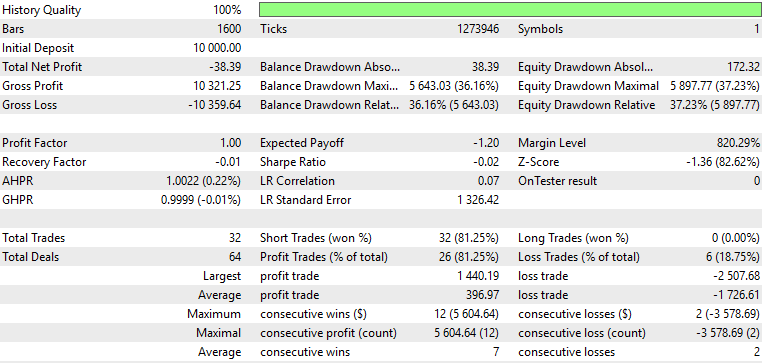
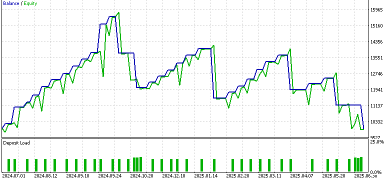
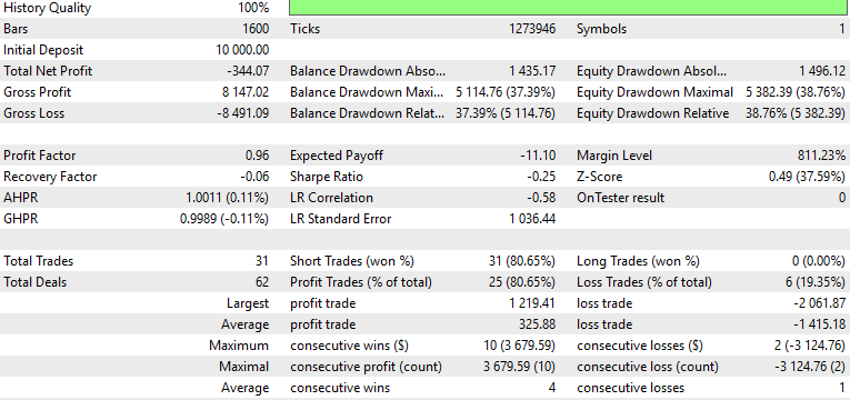
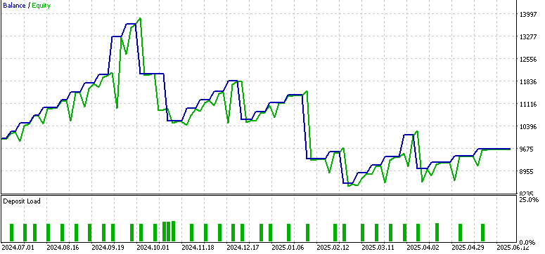
For this article, we conducted three separate tests, one for each of the three signal patterns 0, 1, and 5 from the part-74 article. Each of these patterns had a separate actor network, and this was trained in Python, and then exported by ONNX. All three were trained on the forex symbol EUR USD and on the 4-hour time frame. The training period was 2023.07.01 to 2024.07.01. The subsequent forward walk period was 2024.07.01 to 2025.07.01. We made some changes to the input vector for the networks, besides the use of pipelines, which we are continuing with, from the last article. We are not using a binary format input to the actor network. Recall, in the past when, for instance, we considered adding supervised learning to the signal as a way of better systemizing the Expert Advisor’s signal, the input vector was purely zeros and ones. The presence of a one in any dimension marked that all important metrics for the selected signal pattern were met for with the long signal or the bearish.

For this article, in the interest of exploration, and trying to harness the power of pipelines, we are dabbling again in floating point or vectors with multiple double values as input. So our input vectors track the magnitude of checked indicator readings, and this therefore means that we do not have a standard size for input vectors such as the 2 we had in previous articles. The results are presented below and they have been a far cry from what we got the last time we used binary input vectors with only signal pattern 5 indicating some potential to forward walk.

Pattern-0:

Pattern-1:

Pattern-5:

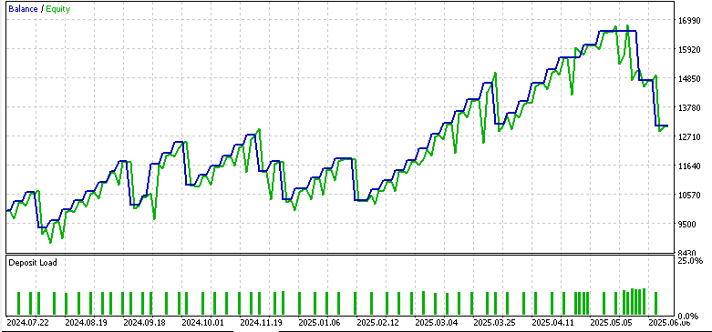
From our reports above it does appear, as pointed out above, that our change of the input features format from binary 0s and 1s to a more continuous version adversely affected our performance. These changes, though, were made to capitalise on our recently introduced data preprocessing, which arguably is important. It can be argued that our choice of the preprocessing implementation in this article could be sub-optimal, therefore in future articles I will look to see how this could be fine tuned.

Conclusion

To wrap up, we have shown here that TD3 can be trained in Python, exported through ONNX, and merged into MQL5 as a custom signal class. Our approach here though, is slightly unorthodoxy because we are using Reinforcement Learning like Supervised Learning in the sense that we do not train/ backpropagate when doing our inference or live trading. Even though this is done in the simulation/ training in Python, RL often requires/ expects this to continue to live deployments.

The forward tests we performed on the signal patterns 0, 1, and 5 revealed that transitioning from binary inputs to continuous feature vectors can be problematic given that only pattern 5 exhibited modestly encouraging results. Even though these results were mixed, they do bring to light the iterative nature of research, which is that subsequent testing brings refinements that draw us closer to robust trading systems. In future articles, optimization of these preprocessing pipelines, more nuanced feature selection, and probably more elaborate forward walks will be under consideration as we make amends.

name	description
WZ-81.mq5	Wizard Assembled Expert Advisor whose header lists referenced files
SignalWZ-81.mqh	Custom Signal Class file used in the wizard assembly
0-1-actor.onnx	Pattern 0 exported network
1-1-actor.onnx	Pattern 1 network
5-1-actor.onnx	Pattern 5 network
PipeLine.mqh	Classes for the different transform types