Neural Networks in Trading: Parameter-Efficient Transformer with Segmented Attention (Final Part)

Introduction

In the previous article, we explored the theoretical aspects of the PSformer framework, which introduces two key innovations into the vanilla Transformer architecture: the Parameter Sharing (PS) mechanism and Spatial-Temporal Segmented Attention (SegAtt).

To recap, the authors of PSformer proposed an encoder based on the Transformer architecture, featuring a two-level segmented attention structure. Each level includes a parameter-sharing block consisting of three fully connected layers with residual connections. This architecture reduces the total number of parameters while maintaining effective information exchange within the model.

Segments are generated using a patching method, where time series variables are divided into patches. Patches with the same position across different variables are grouped into segments, representing a spatial extension of a single-variable patch. This segmentation enables efficient organization of multidimensional time series into multiple segments.

Within each segment, attention focuses on identifying local spatial-temporal relationships, while information integration between segments improves overall forecast quality.

Additionally, the use of SAM optimization methods within the PSformer framework helps reduce the risk of overfitting without compromising performance.

Extensive experiments conducted by the authors on various datasets for long-term time series forecasting confirm the high performance of PSformer. In 6 out of 8 key forecasting tasks, this architecture achieved competitive or superior results compared to state-of-the-art models.

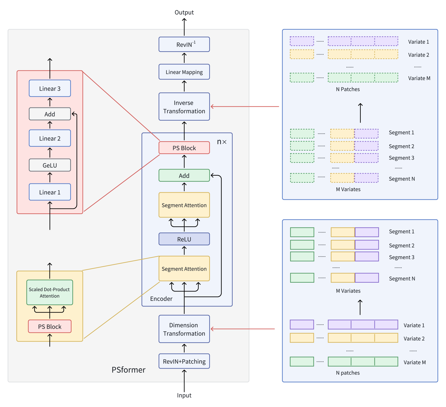
The original visualization of the PSformer framework is provided below.

In the previous article, we started implementing the proposed approaches using MQL5. We examined the algorithms of the CNeuronPSBlock class methods, which implement the parameter-sharing block functionality. We now continue our work and move on to building the encoder functionality.

Creating the PSformer Encoder Object

Before moving to the code implementation, let's briefly discuss the algorithms. According to the framework authors, the input data first passes through RevIn. As you know, the RevIn module consists of two blocks. At the model input, it normalizes the raw data; at the output, it restores the previously extracted distribution parameters to the model results. This helps align the model's output distribution with that of the original data. This is undoubtedly an important factor in forecasting future values of a time series.

In this article, as before, we will only use input data normalization, implemented as a separate batch normalization layer. The reason is that our ultimate goal is not to forecast future time series values, but to train a profitable Actor policy. Since models generally perform better with normalized data, we normalize the input data. For the same reason, it is logical to pass normalized data from the encoder's hidden state to the Actor. Thus, when training the Encoder together with the Actor in the environment, both the linear mapping block and the reverse RevIn module become unnecessary.

Of course, the mapping block and reverse RevIn module are needed in staged training, where the environment state Encoder is first trained to predict subsequent states of the analyzed time series, and only then are the Actor and Critic models trained separately. Even in this case, however, it is preferable to pass the Encoder's hidden state, which contains a more compact and normalized representation of the original data, to the Actor.

Staged training has both advantages and drawbacks. The main advantage is the universality of the Encoder, since it is trained on raw data without being tied to a specific task. This makes it possible to reuse the encoder for solving different problems on the same dataset.

On the other hand, a universal model is not always optimal for a specific task, as it may fail to capture certain domain-specific nuances.

Moreover, two separate training stages may, in total, be more computationally expensive than training all models simultaneously.

Considering these factors, we chose simultaneous training of the models with a reduction of the Encoder architecture.

After data normalization, the PSformer framework applies a patching and data transformation module. The authors describe a rather complex transformation process. Let's try to break it down.

The model receives a multimodal time series as input. Omitting normalization for now, let's focus solely on the transformation process.

First, the multimodal time series is divided into M univariate sequences. Each univariate sequence is then split into N equal patches of length P. Next, patches with identical time indices are combined into segments. This yields N patches of size M×P. 

In our case, the raw data is a sequential description of historical bars over the depth of the analyzed dataset. In other words, our raw data buffer contains M descriptive elements for one bar. These are followed by M elements for the next bar, and so forth. Therefore, to form a segment, we simply need to take P consecutive bar descriptions. Clearly, no additional data transformation is required for this.

The PSformer authors then describe transforming the raw data into (M×P)×N. For our implementation, this can be achieved simply by transposing the input data tensor.

Thus, in our case, the PSformer patching and transformation block is effectively reduced to a single transposition layer.

Another important question is how to build the sequential PSformer encoder layers. There are two options. Use the base approach and specify the desired number of layers directly in the model architecture description or create an object that generates the required number of internal layers.

The first approach complicates architecture description but simplifies Encoder object creation. It also provides flexibility in configuring the Encoder's sequential layers.

The second approach simplifies architecture description but complicates the Encoder implementation, with all internal layers having the same architecture.

Clearly, the first option is preferable for models with a small number of Encoder layers. While the second is more suitable for deeper models.

To decide, we refer to the original study of how the number of encoder layers affects forecasting accuracy. PSformer authors conducted the experiment on standard ETTh1 and ETTm1 time series datasets, which contain data from electrical transformers. Each data point includes eight features such as date, oil temperature, and six types of external load characteristics. ETTh1 has hourly intervals, while ETTm1 has minute intervals. The results are shown in the table below. 

From the presented data, it is clear that for the less chaotic hourly dataset, the best results were achieved with a single Encoder layer. For the noisier minute-level dataset, three Encoder layers proved optimal. Consequently, we do not anticipate building models with a large number of Encoder layers. Therefore, we select the first implementation approach, with a simpler encoder object structure and explicit parameter specification for each encoder layer in the model architecture description.

The complete structure of the new CNeuronPSformer object is shown below.

class CNeuronPSformer   :  public CNeuronBaseSAMOCL
  {
protected:
   CNeuronTransposeOCL           acTranspose[2];
   CNeuronPSBlock                acPSBlocks[3];
   CNeuronRelativeSelfAttention  acAttention[2];
   CNeuronBaseOCL                cResidual;
   //---
   virtual bool      feedForward(CNeuronBaseOCL *NeuronOCL);
   virtual bool      updateInputWeights(CNeuronBaseOCL *NeuronOCL);
   virtual bool      calcInputGradients(CNeuronBaseOCL *NeuronOCL);

public:
                     CNeuronPSformer(void)   {};
                    ~CNeuronPSformer(void)   {};
   //---
   virtual bool      Init(uint numOutputs, uint myIndex, COpenCLMy *open_cl, 
                          uint window, uint units_count, uint segments, float rho, 
                          ENUM_OPTIMIZATION optimization_type, uint batch);
   //---
   virtual int       Type(void)   const         {  return defNeuronPSformer;   }
   //--- methods for working with files
   virtual bool      Save(int const file_handle);
   virtual bool      Load(int const file_handle);
   //---
   virtual CLayerDescription* GetLayerInfo(void);
   virtual void      SetOpenCL(COpenCLMy *obj);
  };

As mentioned earlier, the PSformer framework incorporates SAM optimization techniques. Therefore, our new class inherits the base functionality from the corresponding fully connected layer.

In addition, the CNeuronPSformer structure includes two data transposition layers, which perform the forward and reverse data transformation functions.

The new class structure also contains three parameter-sharing blocks and two relative attention modules, into which we previously integrated SAM optimization functionality. This, perhaps, is our biggest deviation from the original PSformer algorithm.

The authors of PSformer used the parameter-sharing block to generate the Query, Key, and Value entities. In the PS block, parameter matrices have a size of N×N. This implies that the same tensor is used for all three entities.

In our implementation, we slightly complicate the Encoder architecture. The PS block is used solely for preliminary data preparation, while dependency analysis is performed in the more advanced relative attention block.

All internal objects are declared as static, allowing us to keep the class constructor and destructor empty. Initialization of all declared and inherited objects is performed in the Init method. The parameters of this method include key constants that fully define the architecture of the layer being created, namely:

• window — the size of the vector describing one sequence element
• units_count — the depth of the historical data (sequence length)
• segments — the number of generated segments
• rho — the blur region coefficient

bool CNeuronPSformer::Init(uint numOutputs, uint myIndex, COpenCLMy *open_cl,
                           uint window, uint units_count, uint segments, float rho, 
                           ENUM_OPTIMIZATION optimization_type, uint batch)
  {
   if(units_count % segments > 0)
      return false;

Within the initialization method, we first set up a control block to verify that the sequence length is divisible by the number of segments. We then call the parent class method of the same name, which implements further validation of the constants and initialization of inherited objects.

   if(!CNeuronBaseSAMOCL::Init(numOutputs, myIndex, open_cl, window * units_count, rho, optimization_type, batch))
      return false;

Next, we determine the size of a single segment.

   uint count = Neurons() / segments;

We then proceed to initialize the newly declared internal objects. First, we initialize the input data transposition layer. The number of rows in the transposed matrix is set to the number of segments, while the row size is set to the total number of elements in a segment. 

   if(!acTranspose[0].Init(0, 0, OpenCL, segments, count, optimization, iBatch))
      return false;
   acTranspose[0].SetActivationFunction(None);

No activation function is specified for this layer.

While specifying an activation function is not required for a transposition layer, the feed-forward algorithm for this layer provides synchronization with the activation function of the source data object if needed.

Next, we initialize the first parameter-sharing block. For this we use an explicit object initialization method.

   if(!acPSBlocks[0].Init(0, 1, OpenCL, segments, segments, units_count / segments, 1, fRho, optimization, iBatch))
      return false;

We then create a loop to initialize the attention modules and the remaining parameter-sharing blocks.

   for(int i = 0; i < 2; i++)
     {
      if(!acAttention[i].Init(0, i + 2, OpenCL, segments, segments, units_count / segments, 2, optimization, iBatch))
         return false;
      if(!acPSBlocks[i + 1].InitPS((CNeuronPSBlock*)acPSBlocks[0].AsObject()))
         return false;
     }

The remaining parameter-sharing blocks are initialized in the same way as the first PS block, with pointers to the shared parameter buffers and their moments copied accordingly.

Next, we initialize the residual connection recording layer. Here we use a standard fully connected layer, because we only need its data buffers for storing intermediate computation results.

   if(!cResidual.Init(0, 4, OpenCL, acAttention[1].Neurons(), optimization, iBatch))
      return false;
   if(!cResidual.SetGradient(acAttention[1].getGradient(), true))
      return false;
   cResidual.SetActivationFunction((ENUM_ACTIVATION)acAttention[1].Activation());

To reduce data copying operations, we replace the gradient buffer of this layer with that of the final attention module. Ensure that their activation functions are synchronized.

Finally, we initialize the reverse transposition layer.

   if(!acTranspose[1].Init(0, 5, OpenCL, count, segments, optimization, iBatch))
      return false;
   acTranspose[1].SetActivationFunction((ENUM_ACTIVATION)acPSBlocks[2].Activation());

We also replace our object’s interface data buffers with the corresponding buffers of the final transposition layer.

   if(!SetOutput(acTranspose[1].getOutput(), true) ||
      !SetGradient(acTranspose[1].getGradient(), true))
      return false;
//---
   return true;
  }

After this, the initialization method is complete, returning a logical result to the caller.

The next stage is building the feed-forward algorithms, implemented in the feedForward method. This method should be relatively clear since the main functionality resides in the previously implemented internal objects.

The method receives a pointer to the source data object, which is immediately passed to the internal transposition layer for initial transformation. 

bool CNeuronPSformer::feedForward(CNeuronBaseOCL *NeuronOCL)
  {
//--- Dimension Transformation
   if(!acTranspose[0].FeedForward(NeuronOCL))
      return false;

We then iterate through two segment-attention blocks.

//--- Segment Attention
   CObject* prev = acTranspose[0].AsObject();
   for(int i = 0; i < 2; i++)
     {
      if(!acPSBlocks[i].FeedForward(prev))
         return false;
      if(!acAttention[i].FeedForward(acPSBlocks[i].AsObject()))
         return false;
      prev = acAttention[i].AsObject();
     }

Within each loop iteration, we sequentially call the methods of the parameter-sharing block and the relative attention module.

After all iterations of the loop have been successfully completed, we add residual connections to the raw data and save the results in our inner layer buffer cResidual.

//--- Residual Add
   if(!SumAndNormilize(acTranspose[0].getOutput(), acAttention[1].getOutput(), cResidual.getOutput(),
                                                      acAttention[1].GetWindow(), false, 0, 0, 0, 1))
      return false;

But note that for the residual connections we take the raw data after transformation, that is, after the transposition layer. This ensures that the data structure is preserved for residual connections.

The resulting data is then passed through the final parameter-sharing block.

//--- PS Block
   if(!acPSBlocks[2].FeedForward(cResidual.AsObject()))
      return false;

We then perform the reverse data transformation.

//--- Inverse Transformation
   if(!acTranspose[1].FeedForward(acPSBlocks[2].AsObject()))
      return false;
//---
   return true;
  }

Thanks to the shared buffer pointers between our object's interfaces and the final transposition layer, the results of the reverse transformation are written directly to the interface buffers, eliminating the need for additional data copying. Thus, after the reverse transformation, the feed-forward method simply returns a bool result to the caller.

Once the forward pass is complete, we move on to the backward-pass process, implemented in the calcInputGradients and updateInputWeights methods. The former distributes the error gradients, while the latter updates the model parameters.

The calcInputGradients method receives a pointer to the source data object, into which we must pass the error gradient reflecting the impact of the input data on the final result.

bool CNeuronPSformer::calcInputGradients(CNeuronBaseOCL *NeuronOCL)
  {
   if(!NeuronOCL)
      return false;

First, we check the validity of the received pointer - if invalid, further processing is meaningless. Upon passing this check, we sequentially backpropagate the error gradients through the internal layers of our object in the reverse order of the feed-forward pass.

   if(!acPSBlocks[2].calcHiddenGradients(acTranspose[1].AsObject()))
      return false;
//---
   if(!cResidual.calcHiddenGradients(acPSBlocks[2].AsObject()))
      return false;
//---
   if(!acPSBlocks[1].calcHiddenGradients(acAttention[1].AsObject()))
      return false;
   if(!acAttention[0].calcHiddenGradients(acPSBlocks[1].AsObject()))
      return false;
   if(!acPSBlocks[0].calcHiddenGradients(acAttention[0].AsObject()))
      return false;
//---
   if(!acTranspose[0].calcHiddenGradients(acPSBlocks[0].AsObject()))
      return false;

After reaching the input data transformation layer, we must add the residual connection gradient. This may occur in two ways, depending on the activation function of the source data object. If no activation function is present, we simply sum the values from the two data buffers.

   if(acTranspose[0].Activation() == None)
     {
      if(!SumAndNormilize(acTranspose[0].getGradient(), cResidual.getGradient(), acTranspose[0].getGradient(),
                                                               acAttention[1].GetWindow(), false, 0, 0, 0, 1))
         return false;
     }

If an activation function exists, we first adjust the error gradient by the derivative of the activation function before summing the data.

   else
     {
      if(!DeActivation(acTranspose[0].getOutput(), cResidual.getGradient(), acTranspose[0].getPrevOutput(),
                                                                                     acTranspose[0].Activation()) ||
         !SumAndNormilize(acTranspose[0].getGradient(), acTranspose[0].getPrevOutput(), acTranspose[0].getGradient(), 
                                                                      acAttention[1].GetWindow(), false, 0, 0, 0, 1))
         return false;
     }

At the end of the method, we perform the reverse transformation to propagate the error gradient to the input level, and then return the bool result to the calling program.

   if(!NeuronOCL.calcHiddenGradients(acTranspose[0].AsObject()))
      return false;
//---
   return true;
  }

To complete the backpropagation pass, we must update the model parameters to reduce the forecasting error. Recall that we use SAM optimization techniques for parameter updates. As discussed earlier, SAM requires a second forward pass with perturbed model parameters, which changes the buffer values. While this does not affect the current layer operations, it can distort parameter updates in subsequent layers. Therefore, we update the internal layers in reverse feed-forward pass order. This allows adjusting each layer's parameters before any buffer values from preceding layers are modified.

bool CNeuronPSformer::updateInputWeights(CNeuronBaseOCL *NeuronOCL)
  {
   if(!acPSBlocks[2].UpdateInputWeights(cResidual.AsObject()))
      return false;
//---
   CObject* prev = acAttention[0].AsObject();
   for(int i = 1; i >= 0; i--)
     {
      if(!acAttention[i].UpdateInputWeights(acPSBlocks[i].AsObject()))
         return false;
      if(!acPSBlocks[i].UpdateInputWeights(prev))
         return false;
      prev = acTranspose[0].AsObject();
     }
//---
   return true;
  }

A few words should be said about file operation methods. Since we use three parameter-sharing blocks, there is no need to save the same parameters three times. Saving them once is sufficient. Accordingly, we have the following Save method.

The method receives a file handle, which is first passed to the Save method of the parent class.

bool CNeuronPSformer::Save(const int file_handle)
  {
   if(!CNeuronBaseSAMOCL::Save(file_handle))
      return false;

We then save the parameter-sharing block once.

   if(!acPSBlocks[0].Save(file_handle))
      return false;

Next, we loop to save the attention modules and transposition layers.

   for(int i = 0; i < 2; i++)
      if(!acTranspose[i].Save(file_handle) ||
         !acAttention[i].Save(file_handle))
         return false;
//---
   return true;
  }

After completing the loop, we return the bool result to the caller and finish the method.

Note that when saving, we also omit the residual connection layer. It has no trainable parameters. Therefore, no information is lost in this process.

However, when restoring a previously saved object, we must also restore the structure and functionality of all objects. Including those skipped during saving. Therefore, I suggest taking a closer look at the Load method that restores object functionality.

In the method parameters, we receive the file handle with previously saved data. We immediately pass the received handle to the Load method of the parent class, which restores the inherited objects.

bool CNeuronPSformer::Load(const int file_handle)
  {
   if(!CNeuronBaseSAMOCL::Load(file_handle))
      return false;

We then restore the saved objects in the exact order they were saved.

   if(!LoadInsideLayer(file_handle, acPSBlocks[0].AsObject()))
      return false;
   for(int i = 0; i < 2; i++)
      if(!LoadInsideLayer(file_handle, acTranspose[i].AsObject()) ||
         !LoadInsideLayer(file_handle, acAttention[i].AsObject()))
         return false;

Then we need to restore the functionality of the objects missed during saving. First we will restore the parameter-sharing blocks. One is loaded from the file, and others are initialized based on the loaded block and copying pointers to the shared parameter buffers and their moments.

   for(int i = 1; i < 3; i++)
      if(!acPSBlocks[i].InitPS((CNeuronPSBlock*)acPSBlocks[0].AsObject()))
         return false;

We also initialize the residual connection recording layer. Its size is equal to the output tensor of the final relative attention module.

   if(!cResidual.Init(0, 4, OpenCL, acAttention[1].Neurons(), optimization, iBatch))
      return false;
   if(!cResidual.SetGradient(acAttention[1].getGradient(), true))
      return false;
   cResidual.SetActivationFunction((ENUM_ACTIVATION)acAttention[1].Activation());

We replace the gradient buffer pointer to eliminate unnecessary copying operations and synchronize activation functions.

Finally, we replace our object's interface buffers with those of the last transposition layer.

   if(!SetOutput(acTranspose[1].getOutput(), true) ||
      !SetGradient(acTranspose[1].getGradient(), true))
      return false;
//---
   return true;
  }

The method concludes by returning the logical result of the operation to the caller.

At this point, our work on the CNeuronPSformer encoder object is complete. You can find the full code of this class and all its methods in the attachment.

Model Architecture

After constructing objects that implements the approaches proposed by the authors of the PSformer framework, we move on to the description of the architecture of the trainable models. First of all, we are interested in the environmental state Encoder, into which we implement the proposed approaches.

The architecture of the Environmental State Encoder is defined in the CreateEncoderDescriptions method. In the method parameters, we pass a pointer to a dynamic array object for recording the description of the model architecture.

bool CreateEncoderDescriptions(CArrayObj *&encoder)
  {
//---
   CLayerDescription *descr;
//---
   if(!encoder)
     {
      encoder = new CArrayObj();
      if(!encoder)
         return false;
     }

In the method body, we check the relevance of the received pointer and, if necessary, create a new instance of the dynamic array.

As before, the raw data layer is a standard fully connected layer. Its size must be enough to capture the full historical data tensor for the specified analysis depth.

//--- Encoder
   encoder.Clear();
//--- Input layer
   if(!(descr = new CLayerDescription()))
      return false;
   descr.type = defNeuronBaseOCL;
   int prev_count = descr.count = (HistoryBars * BarDescr);
   descr.activation = None;
   descr.optimization = ADAM;
   if(!encoder.Add(descr))
     {
      delete descr;
      return false;
     }

This is followed by a batch normalization layer for initial preprocessing of the raw data.

//--- layer 1
   if(!(descr = new CLayerDescription()))
      return false;
   descr.type = defNeuronBatchNormOCL;
   descr.count = prev_count;
   descr.batch = 1e4;
   descr.activation = None;
   descr.optimization = ADAM;
   if(!encoder.Add(descr))
     {
      delete descr;
      return false;
     }

The normalized data is then passed to the PSformer encoder. In this article, we use three sequential PSformer encoder layers with identical architectures. To define the required number of encoder layers, we use a loop whose iteration count equals the desired encoder depth. In the body of the loop, at each iteration, we create a description of one CNeuronPSformer object.

//--- layer 2 - 4
   for(int i = 0; i < 3; i++)
     {
      if(!(descr = new CLayerDescription()))
         return false;
      descr.type = defNeuronPSformer;
      descr.window = BarDescr;
      descr.count = HistoryBars;
      descr.window_out = Segments;
      descr.probability = Rho;
      descr.batch = 1e4;
      descr.activation = None;
      descr.optimization = ADAM;
      if(!encoder.Add(descr))
        {
         delete descr;
         return false;
        }
     }

After the PSformer encoder, we apply a mapping block consisting of one convolutional and one fully connected layer. All neural layers are adapted for SAM optimization.

//--- layer 5
   if(!(descr = new CLayerDescription()))
      return false;
   descr.type = defNeuronConvSAMOCL;
   descr.count = HistoryBars;
   descr.window = BarDescr;
   descr.step = BarDescr;
   descr.window_out = int(LatentCount / descr.count);
   descr.probability = Rho;
   descr.activation = GELU;
   descr.optimization = ADAM;
   if(!encoder.Add(descr))
     {
      delete descr;
      return false;
     }
//--- layer 6
   if(!(descr = new CLayerDescription()))
      return false;
   descr.type = defNeuronBaseSAMOCL;
   descr.count = LatentCount;
   descr.probability = Rho;
   descr.activation = None;
   descr.optimization = ADAM;
   if(!encoder.Add(descr))
     {
      delete descr;
      return false;
     }
//---
   return true;
  }

Once the architecture description for the environment state encoder is complete, we return the bool result to the caller and exit the method.

The full code for this method describing the Encoder architecture is provided in the attachment, along with the unchanged Actor and Critic model architectures from previous articles.

We also carried over, without modification, the environment interaction and model training programs. They are also available in the attachment. We now proceed to the final stage - evaluating the effectiveness of the implemented techniques on real historical data.

Testing

We have done quite a lot of work to implement the approaches proposed by the PSformer framework authors using MQL5. Now comes the most exciting stage - evaluating their effectiveness on real-world historical data.

It is important to emphasize that this is an evaluation of our implemented techniques, not merely those proposed by the original authors. Because our implementation includes certain deviations from the original PSformer framework.

We trained the models on EURUSD historical data for the entirety of 2023 on the H1 timeframe. As always, all indicator parameters were set to their default values.

As noted earlier, the environment state encoder, Actor, and Critic models were trained simultaneously. For initial training, we used a dataset collected while working with previous models, updating it periodically as training progressed.

After several iterations of model training and dataset updates, we obtained a policy capable of generating profit on both the training and test datasets.

The trained Actor policy was tested on EURUSD historical data from January 2024, keeping all other parameters unchanged. The test results are presented below.

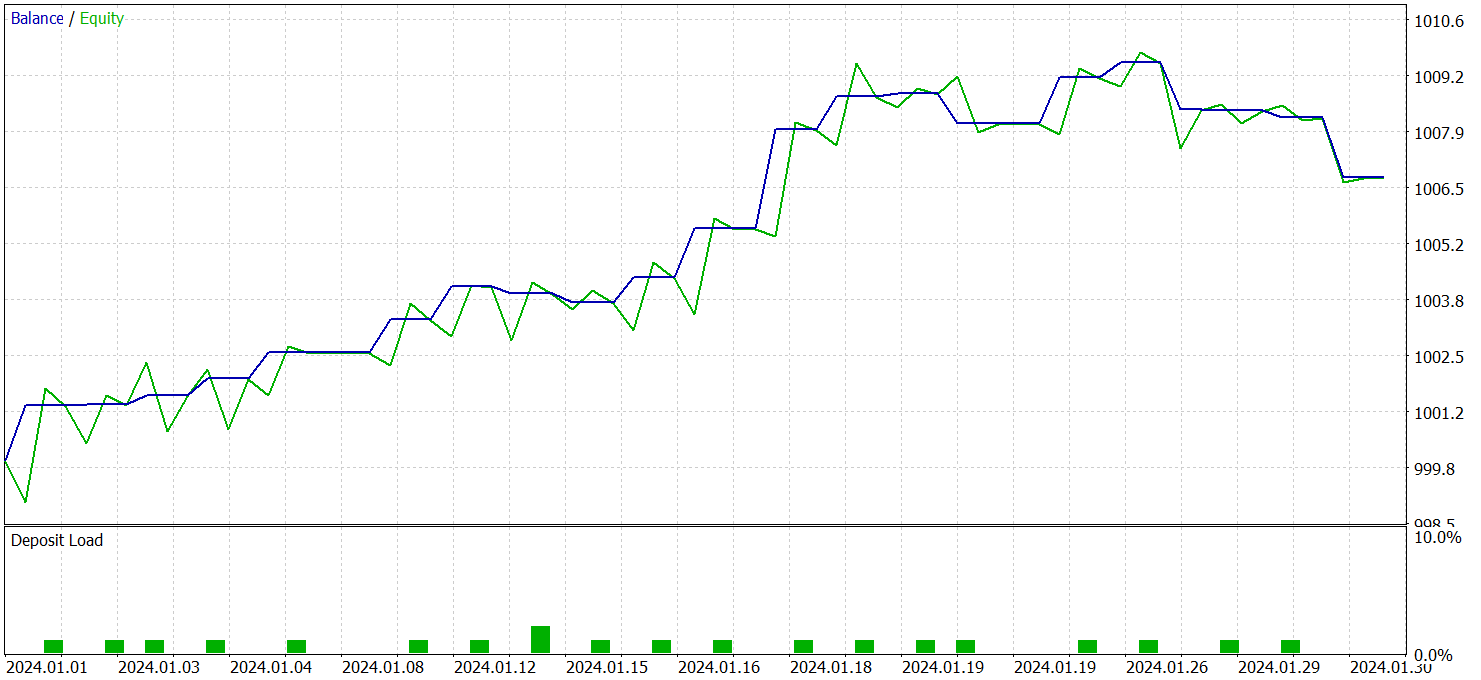
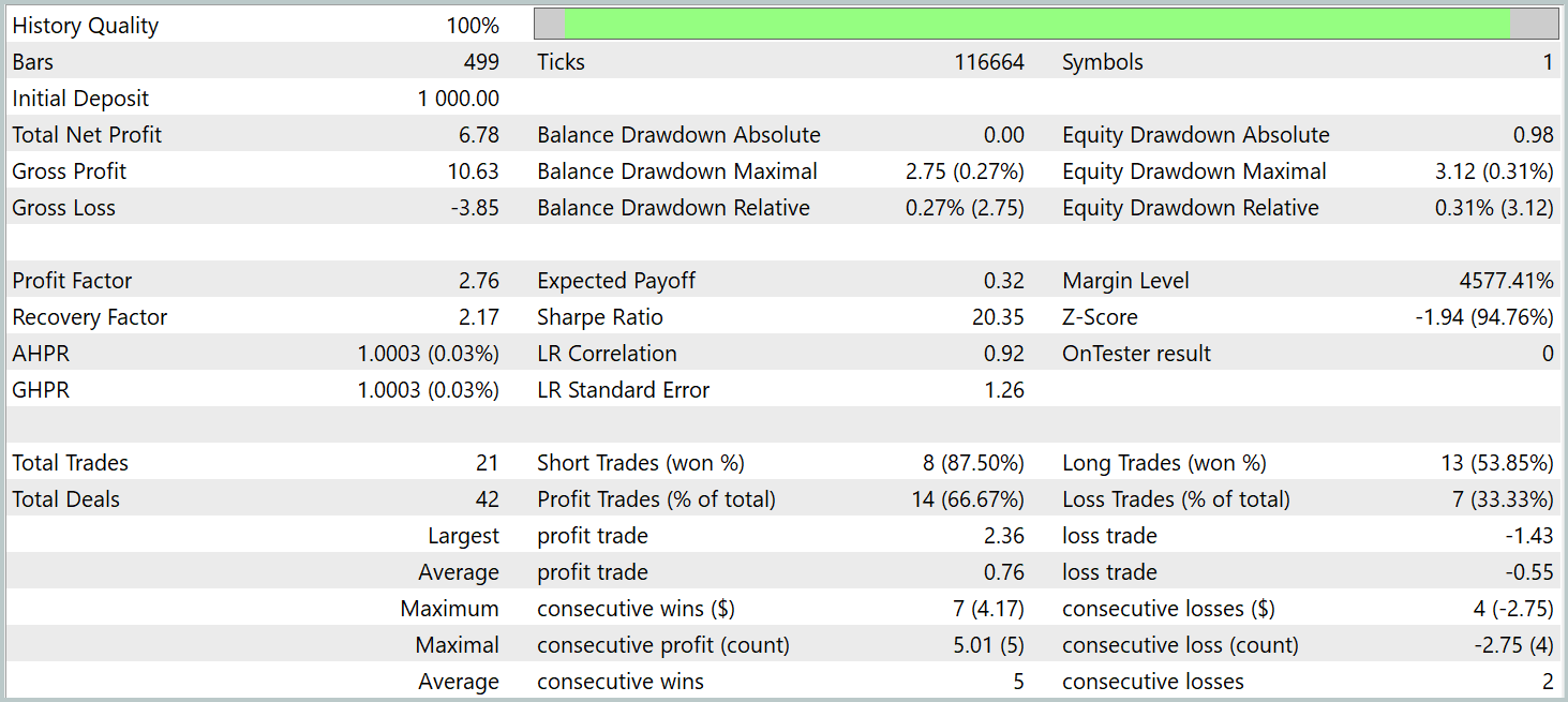
During the test period, the model executed 21 trades, i.e., an average of approximately one trade per trading day. Of these, 14 were profitable, representing over 66%. The average profitable trade exceeded the average losing trade by 38%.

The balance graph shows a clear upward trend during the first two decades of the month.

Overall, the results demonstrate promising potential. With further refinement and additional training on a larger dataset, the model could be used for live trading.

Conclusion

We have explored the PSformer framework, noted for its high accuracy in time series forecasting and efficient computational resource usage. The key architectural elements of PSformer include the Parameter Sharing (PS) block and Spatial-Temporal Segmented Attention (SegAtt) mechanism. These elements enable effective modeling of both local and global time series dependencies while reducing parameter count without sacrificing forecast quality.

We have implemented our own interpretation of the proposed approaches in MQL5. We trained models using these methods, and tested them on historical data outside the training set. The results indicate clear potential for the trained models.

References

PSformer: Parameter-efficient Transformer with Segment Attention for Time Series Forecasting

Other articles from this series

Programs used in the article

#	Name	Type	Description
1	Research.mq5	Expert Advisor	Expert Advisor for collecting examples
2	ResearchRealORL.mq5	Expert Advisor	Expert Advisor for collecting examples using the Real-ORL method
3	Study.mq5	Expert Advisor	Model training Expert Advisor
4	StudyEncoder.mq5	Expert Advisor	Encoder training Expert Advisor
5	Test.mq5	Expert Advisor	Model testing Expert Advisor
6	Trajectory.mqh	Class library	System state description structure
7	NeuroNet.mqh	Class library	A library of classes for creating a neural network
8	NeuroNet.cl	Library	OpenCL program code library