Price Action Analysis Toolkit Development (Part 35): Training and Deploying Predictive Models

Introduction

In the preceding article, we established a reliable pipeline for streaming historical data from an MQL5 script into Python and persisting it on disk. That piece intentionally stopped at the ingestion layer; we proved that market bars can be captured, serialized, and reloaded, but we did not proceed to model fitting.

This instalment picks up exactly where we left off. We move beyond storage and show how to:

• train predictive models on the ingested data,
• package and cache those models per symbol, and
• deploy them behind a lightweight REST API that an MQL5 Expert Advisor can query in real time.

To achieve this, we combine the strengths of Python’s machine-learning ecosystem with the execution speed of MetaTrader 5. The EA handles market interaction, while the Python service performs feature engineering, model inference, and—optionally—periodic retraining.

A “trainable model” in this context is any algorithm whose internal parameters can be optimised from data. Classical techniques (via scikit-learn) such as Gradient Boosting or Support-Vector Machines are suitable for tabular feature sets, whereas deep-learning frameworks (TensorFlow, PyTorch) support more complex architectures when required. Python’s extensive library support, clear syntax, and active community make it the language of choice for this stage of the pipeline.

The table below summarizes the respective responsibilities in the finished system:

Component	Role in the Workflow
MQL5 Expert Advisor	Gathers live bars and account state; sends feature requests; executes trade signals returned by the API.
Python Ingestion Script	Receives historical chunks from MetaTrader 5, cleans and stores them (Parquet).
Feature-engineering module	Converts raw OHLC data into technical and statistical features.
Training Module	Fits or updates per-symbol models; serializes them with joblib.
flask REST services	Serves /predict, /upload_history, etc.; manages an in-memory model cache for millisecond-level responses.

This article is organized as follows:

• Introduction
• Recap of the Ingestion Pipeline
• MQL5 and Python Implementation
• Model training in Python
• Model deployment and real-time inference
• Conclusion

Let’s dive in.

Recap of the Ingestion Pipeline

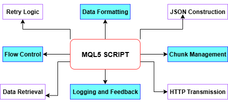
As covered in the previous article, our history ingestion script streamlines the entire MetaTrader 5‑to‑Python workflow: it first pulls the desired historical bars via CopyRates, then parses timestamps, highs, lows, and closes into arrays before assembling each portion into a JSON payload with BuildJSON. To stay within MetaTrader 5’s WebRequest size limits, it automatically splits the data into manageable chunks—halving chunk sizes as needed down to a defined minimum—and dispatches each slice to our Python endpoint using PostChunk, complete with retry logic and timeout controls. Along the way, it logs every step and error in the Experts tab and exits cleanly on failure or confirms completion once all data is uploaded, laying a rock‑solid foundation for our spike‑detection pipeline.

Let’s examine the diagram below to explore each function within the MQL5 script.

On the python side, the ingestion pipeline consists of four key components: the HTTP Receiver (upload_history) parses each JSON chunk sent from the MQL5 script, extracting symbols, timestamps, and price data; the Feature Enricher (prophet_delta backed by _compile_prophet) maintains a cached Prophet model per symbol to generate forecast deltas on the fly; the Feature Calculator (within upload_history) computes a suite of technical metrics—spike magnitude, MACD, RSI, ATR, envelope bands, Kalman slope, etc.—and assigns a “BUY/SELL/WAIT” label; and finally the Data Persister (append_rows) writes these enriched, labeled rows into training_set.csv, creating the file and header if they don’t already exist.

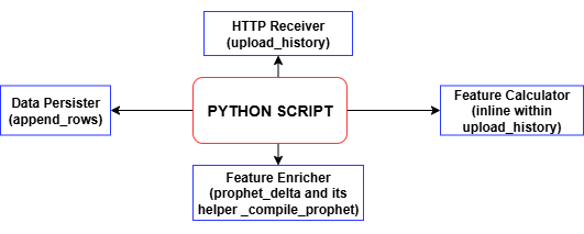
Each time the MQL5 script posts a chunk of historical bars, the Python endpoint’s upload_history handler computes all the technical features and labels, then calls append_rows to write those records into training_set.csv—creating the file and header if they don’t already exist. With each successive upload, you build a complete, timestamped dataset that’s ready for model training. This training_set.csv is undoubtedly what we’ll use to train our spike‑detection model.

MQL5 and Python Implementation

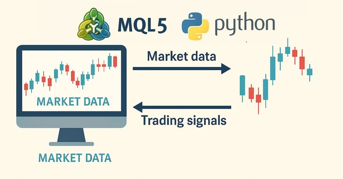
In this article, we transition from using a simple script to developing a full Expert Advisor (EA) to allow continuous monitoring and real-time communication with a Python backend—something a standalone script cannot efficiently handle. The Spike Detector EA on MetaTrader 5 operates in a client-server setup, where it serves as the client and a Python Flask server acts as the backend. The EA continuously observes the formation of new candlesticks. At defined intervals, it collects a configured number of historical candles (OHLCV data and timestamps), serializes this into JSON format, and sends it via an HTTP POST request to the Python server.

The Python backend, which typically contains either a machine learning model or rule-based logic, analyzes the incoming market data and returns a signal: BUY, SELL, CLOSE, or WAIT. Upon receiving this response, the EA interprets the signal and reacts accordingly—drawing arrows on the chart, opening trades, or closing existing positions—based on the user’s settings. This feedback loop allows MetaTrader to extend its native capabilities with external analytical intelligence in real time, effectively combining MetaTrader 5's execution engine with Python's processing power.

MQL5 Implementation

Script Metadata and Strict Mode

At the very top of your MQL5 file, you declare metadata properties—such as #property copyright, #property link, and #property version—to embed authorship and version information directly into the compiled EA. Enabling #property strict enforces the most rigorous compile‑time checks, helping you catch syntax or type errors early and ensuring your code adheres to best practices.

#property copyright "Copyright 2025, MetaQuotes Ltd."
#property link      "https://www.mql5.com/en/users/lynnchris"
#property version   "1.0"
#property strict

Importing the Trading Library

By including <Trade\Trade.mqh> and instantiating a CTrade object, you gain access to MetaTrader’s native trade‑management API. This built‑in library exposes methods for market orders, stop orders, position closing, and other essential operations, so you can open, modify, and close trades programmatically in response to your server’s signals.

#include <Trade\Trade.mqh>
static CTrade trade;

Defining Input Parameters

All user‑configurable settings—from the REST endpoint URL (InpServerURL) and the number of bars to send (InpBufferBars), to chart‑drawing options and trade‑execution flags—are declared up front with input statements. Each parameter includes an inline comment explaining its purpose, which makes the EA self‑documenting and allows traders to fine‑tune behavior directly in the MetaTrader 5 GUI without touching code.

// REST endpoint & polling
input string InpServerURL      = "http://127.0.0.1:5000/analyze";
input int    InpBufferBars     = 200;
input int    MinSecsBetweenReq = 10;

// Visual & trading options
input color  ColorBuy          = clrLime;
input color  ColorSell         = clrRed;
input bool   DrawSLTPLines     = true;
input bool   EnableTrading     = true;
input double FixedLots         = 0.10;

// Debug & retry controls
input int    MaxRetry          = 3;
input bool   DebugPrintJSON    = true;
input bool   DebugPrintReply   = true;

Global State Variables

You maintain several globals—such as lastBarTime and lastReqTime to throttle requests, retryCount for your HTTP retry logic, and _digits plus tickSize for precise price formatting. An objPrefix string, seeded with the current chart’s ID, namespaces all chart objects (arrows and lines) created by this EA so that they can be cleanly identified and removed later.

datetime lastBarTime = 0;
datetime lastReqTime = 0;
int      retryCount  = 0;
int      _digits;
double   tickSize;
string   objPrefix;

Initialization in OnInit

When the EA starts, OnInit() runs once to validate inputs (e.g. ensuring at least two bars are requested), cache symbol properties (SYMBOL_DIGITS and SYMBOL_POINT), and generate a unique object‑prefix. A startup message logs the number of bars to be posted and the target server URL, confirming the EA is ready to begin its polling cycle.

int OnInit()
{
   if(InpBufferBars < 2)
      return INIT_FAILED;

   _digits   = (int)SymbolInfoInteger(_Symbol, SYMBOL_DIGITS);
   tickSize  = SymbolInfoDouble(_Symbol, SYMBOL_POINT);
   objPrefix = StringFormat("SpikeEA_%I64d_", ChartID());

   PrintFormat("[SpikeEA] Initialized: posting %d bars → %s",
               InpBufferBars, InpServerURL);
   return INIT_SUCCEEDED;
}

Cleanup in OnDeinit

Upon removal or shutdown, OnDeinit() iterates backward through all chart objects and deletes those whose names begin with your objPrefix. This guarantees that no stray arrows or SL/TP lines linger on the chart after the EA is deactivated, leaving your workspace clean.

void OnDeinit(const int reason)
{
   for(int i = ObjectsTotal(0) - 1; i >= 0; --i)
   {
      string name = ObjectName(0, i);
      if(StringFind(name, objPrefix) == 0)
         ObjectDelete(0, name);
   }
}

Polling and Payload Construction in OnTick

On each tick, the EA checks whether a new bar has formed (if PollOnNewBarOnly is enabled) and ensures a minimum interval (MinSecsBetweenReq) has elapsed since the last request. It then pulls the last InpBufferBars via CopyRates, arranges them in series order, and invokes BuildJSON() to serialize closes and timestamps into the JSON payload. If debugging is active, the raw JSON is printed to the Experts log before being sent.

void OnTick()
{
   datetime barTime = iTime(_Symbol, _Period, 0);
   if(barTime == lastBarTime) return;
   lastBarTime = barTime;

   if(TimeCurrent() - lastReqTime < MinSecsBetweenReq) return;

   MqlRates rates[];
   if(CopyRates(_Symbol, _Period, 0, InpBufferBars, rates) != InpBufferBars)
      return;
   ArraySetAsSeries(rates, true);

   string payload = BuildJSON(rates);
   if(DebugPrintJSON) PrintFormat("[SpikeEA] >>> %s", payload);

   SServerMsg msg;
   if(CallServer(payload, msg))
      ActOnSignal(msg);

   lastReqTime = TimeCurrent();
}

Building JSON in BuildJSON

The helper BuildJSON() takes the array of MqlRates and constructs a compact JSON string containing your symbol name, an array of close prices (formatted to the correct number of decimal places), and a parallel array of UNIX‑style timestamps. String escaping is applied to handle any special characters in the symbol name, ensuring valid JSON output.

string BuildJSON(const MqlRates &r[])
{
   string j = StringFormat("{\"symbol\":\"%s\",\"prices\":[", _Symbol);
   for(int i = 0; i < InpBufferBars; i++)
      j += DoubleToString(r[i].close, _digits) + (i+1<InpBufferBars?",":"");
   j += "],\"timestamps\":[";
   for(int i = 0; i < InpBufferBars; i++)
      j += IntegerToString(r[i].time) + (i+1<InpBufferBars?",":"");
   j += "]}";
   return j;
}

Server Communication in CallServer

CallServer() converts the JSON string into a uchar[] buffer, then performs an HTTP POST to InpServerURL using WebRequest(). It handles timeouts and non‑200 status codes with retry logic up to MaxRetry, printing errors if requests fail. On success, it captures the raw text reply—optionally logging it—and passes it to ParseJSONLite() for interpretation.

bool CallServer(const string &payload, SServerMsg &out)
{
   uchar body[];
   int len = StringToCharArray(payload, body, 0, WHOLE_ARRAY, CP_UTF8);
   ArrayResize(body, len);

   string hdr = "Content-Type: application/json\r\n";
   uchar reply[]; string resp_hdr;
   int status = WebRequest("POST", InpServerURL, hdr,
                           InpTimeoutMs, body, reply, resp_hdr);

   if(status <= 0)
   {
      PrintFormat("WebRequest error %d (retry %d/%d)",
                  GetLastError(), retryCount+1, MaxRetry);
      ResetLastError();
      if(++retryCount >= MaxRetry) retryCount = 0;
      return false;
   }
   retryCount = 0;

   string resp = CharArrayToString(reply);
   if(DebugPrintReply)
      PrintFormat("[SpikeEA] <<< HTTP %d – %s", status, resp);
   if(status != 200) return false;

   return ParseJSONLite(resp, out);
}

Lightweight JSON Parsing in ParseJSONLite

Instead of a full JSON library, ParseJSONLite() employs simple string searches (StringFind) to detect keywords like "signal":"BUY" and numeric keys such as "conf":, "sl":, and "tp":.

bool ParseJSONLite(const string &txt, SServerMsg &o)
{
   o.code = SIG_WAIT; o.conf = o.sl = o.tp = 0.0;

   if(StringFind(txt, "\"signal\":\"BUY\"")   >= 0) o.code = SIG_BUY;
   if(StringFind(txt, "\"signal\":\"SELL\"")  >= 0) o.code = SIG_SELL;
   if(StringFind(txt, "\"signal\":\"CLOSE\"") >= 0) o.code = SIG_CLOSE;

   // extract numeric values
   ParseJSONDouble(txt, "\"conf\":", o.conf);
   ParseJSONDouble(txt, "\"sl\":",   o.sl);
   ParseJSONDouble(txt, "\"tp\":",   o.tp);

   return true;
}

It extracts and converts these substrings into the SServerMsg structure, setting the EA’s signal code, confidence value, stop‑loss, and take‑profit levels.

void ParseJSONDouble(const string &txt, const string &key, double &out)
{
   int p = StringFind(txt, key);
   if(p >= 0)
      out = StringToDouble(StringSubstr(txt, p + StringLen(key)));
}

Acting on Signals in ActOnSignal

When a new signal arrives, ActOnSignal() first clears any previous arrows or lines by matching your objPrefix. It then draws a new arrow at the current bid price—choosing icon code, color, and size based on the signal type—and, if enabled, adds horizontal SL and TP lines with labels. Finally, if live trading is turned on, it uses the trade object to open or close positions according to the signal: Buy(), Sell(), or PositionClose().

void ActOnSignal(const SServerMsg &m)
{
   static ESignal last = SIG_WAIT;
   if(m.code == SIG_WAIT || m.code == last) return;
   last = m.code;

   // remove old objects
   for(int i=ObjectsTotal(0)-1;i>=0;--i)
      if(StringFind(ObjectName(0,i),objPrefix)==0)
         ObjectDelete(0,ObjectName(0,i));

   // draw arrow
   int    arrow = (m.code==SIG_BUY ? 233 : m.code==SIG_SELL ? 234 : 158);
   color  clr   = (m.code==SIG_BUY ? ColorBuy : m.code==SIG_SELL ? ColorSell : ColorClose);
   string id    = objPrefix + "Arr_" + TimeToString(TimeCurrent(),TIME_SECONDS);
   double y     = SymbolInfoDouble(_Symbol, SYMBOL_BID);
   if(ObjectCreate(0,id,OBJ_ARROW,0,TimeCurrent(),y))
   {
      ObjectSetInteger(0,id,OBJPROP_ARROWCODE,arrow);
      ObjectSetInteger(0,id,OBJPROP_COLOR,clr);
      ObjectSetInteger(0,id,OBJPROP_WIDTH,ArrowSize);
      PlaySound("alert.wav");
   }

   // draw SL/TP lines
   if(DrawSLTPLines && m.sl>0)
      ObjectCreate(0,objPrefix+"SL_"+id,OBJ_HLINE,0,0,m.sl);
   if(DrawSLTPLines && m.tp>0)
      ObjectCreate(0,objPrefix+"TP_"+id,OBJ_HLINE,0,0,m.tp);

   // execute trade
   if(EnableTrading)
   {
      bool hasPos = PositionSelect(_Symbol);
      if(m.code==SIG_BUY  && !hasPos) trade.Buy(FixedLots,_Symbol,0,m.sl,m.tp);
      if(m.code==SIG_SELL && !hasPos) trade.Sell(FixedLots,_Symbol,0,m.sl,m.tp);
      if(m.code==SIG_CLOSE&&  hasPos) trade.PositionClose(_Symbol,SlippagePoints);
   }
}

Compilation and Deployment

To finalize, paste the EA code into MetaEditor, save it under Experts, and press F7. After confirming “0 errors, 0 warnings,” switch back to MetaTrader 5, locate your EA in the Navigator, drag it onto a chart, and configure inputs in the popup dialog. The Experts and Journal tabs will then display real‑time logs of JSON POSTs, parsed signals, drawn objects, and any trade executions.

Python Implementation

File Header & Requirements

At the very top of engine.py, we include a Unix shebang (#!/usr/bin/env python3) and a descriptive comment block summarizing the back‑end’s capabilities—vectorized history ingestion, CSV normalization, Prophet caching, training, backtesting, and CLI modes—along with the pip install command for all required dependencies. This header not only documents what the script does at a glance but also provides any developer with the exact list of libraries needed to run the system out of the box.

#!/usr/bin/env python3
# engine.py – Boom/Crash/Vol-75 ML back-end
# • vectorised /upload_history
# • /upload_spike_csv
# • Prophet cache (1h)
# • robust CSV writer
# • train() drops bad rows
# • SL/TP with ATR or fallback
# • backtest defaults to 30 days
# • CLI: collect · history · train · backtest · serve · info
#
# REQS: pip install numpy pandas ta prophet cmdstanpy pykalman \
#            scikit-learn flask MetaTrader5 joblib pytz

User‑Configurable Settings

Immediately after the header, we define constants for terminal login details (TERM_PATH, LOGIN, PASSWORD, SERVER) and an array of SYMBOLS that our system will process. We also set parameters controlling look‑ahead for labeling (LOOKAHEAD, THRESH_LABEL), polling intervals (STEP_SECONDS), thresholds for opening and closing trades (THR_BC_OPEN, THR_O_OPEN, THR_O_CLOSE), and ATR‑based stop‑loss/take‑profit multipliers (ATR_PERIOD, SL_MULT, TP_MULT, ATR_FALLBACK_P). By centralizing these values, users can quickly tailor the strategy’s risk parameters, data windows, and symbol list without diving into code logic.

TERM_PATH  = r""
LOGIN      = 123456
PASSWORD   = "passwd"
SERVER     = "DemoServer"

SYMBOLS = [
    "Boom 900 Index",  "Crash 1000 Index",
    "Volatility 75 (1s) Index"
]

LOOKAHEAD    = 10       # minutes
THRESH_LABEL = 0.0015   # 0.15 %
STEP_SECONDS = 60       # live collect interval

ATR_PERIOD     = 14
SL_MULT        = 1.0
TP_MULT        = 2.0
ATR_FALLBACK_P = 0.002

File Paths & CSV Header

Next, we establish file‑system constants: BASE_DIR as the root analysis folder, CSV_FILE pointing to our aggregated training dataset, MODEL_DIR for per‑symbol model artifacts, and GLOBAL_PKL for the catch‑all model. We also define CSV_HEADER, a fixed list of column names ensuring every row written has the same 12 fields. This section standardizes where data lives and enforces consistency in our stored CSV, which is critical for seamless downstream training and analysis.

BASE_DIR   = r"C:\Analysis EA"
CSV_FILE   = rf"{BASE_DIR}\training_set.csv"
MODEL_DIR  = rf"{BASE_DIR}\models"
GLOBAL_PKL = rf"{MODEL_DIR}\_global.pkl"

CSV_HEADER = [
    "timestamp","symbol","price","spike_mag","macd","rsi",
    "atr","slope","env_low","env_up","delta","label"
]

Imports & Logging Setup

We import standard libraries (os, sys, time, threading, etc.), data‑science packages (numpy, pandas, ta, joblib), the Prophet and Kalman‑filter modules, Flask for our API, and the MetaTrader 5 Python wrapper. Warnings are suppressed for cleanliness, and logging is configured to print timestamps, log levels, and messages in a human‑readable format. Finally, we ensure the model directory exists and change the working directory to BASE_DIR, so all relative file operations happen in one known location.

import os,sys,time,logging,warnings,argparse,threading,io
import datetime as dt
from pathlib import Path
import numpy as np, pandas as pd, ta, joblib, pytz
from flask import Flask, request, jsonify, abort
from prophet import Prophet
from pykalman import KalmanFilter
import MetaTrader5 as mt5

warnings.filterwarnings("ignore")
logging.basicConfig(level=logging.INFO,
                    format="%(asctime)s %(levelname)-7s %(message)s",
                    datefmt="%H:%M:%S")
Path(MODEL_DIR).mkdir(parents=True, exist_ok=True)
os.chdir(BASE_DIR)

MetaTrader 5 Initialization Helpers

The init_mt5() function safely initializes the MetaTrader 5 connection, first trying a default call and falling back to credentials if needed; failure triggers a clean exit with an error message. ensure_symbol(sym) simply wraps mt5.symbol_select to guarantee each instrument is active before data requests. A threading lock (_mt5_lock) protects any multi‑threaded calls to MetaTrader 5, preserving thread safety when our server spawns background tasks.

_mt5_lock = threading.Lock()
def init_mt5():
    if mt5.initialize(): return
    if not mt5.initialize(path=TERM_PATH, login=LOGIN,
                          password=PASSWORD, server=SERVER):
        sys.exit(f"MT5 init failed {mt5.last_error()}")

def ensure_symbol(sym):
    return mt5.symbol_select(sym, True)

Prophet Cache & Forecast Delta

To avoid recompiling the Prophet model on every request, we maintain a thread‑safe dictionary _PROP mapping symbols to either None (compile pending) or a (model, timestamp) tuple. _compile_prophet(df, sym) trains a new Prophet model on historical data and records the time. prophet_delta(prices, times, sym) checks the cache: if missing or stale (over one hour), it launches a background compile; if already available, it forecasts one second ahead and returns the predicted delta. This design keeps forecasting responsive and avoids blocking incoming requests.

_PROP_LOCK = threading.Lock()
_PROP = {}  # sym -> (model, timestamp) or None

def _compile_prophet(df, sym):
    mdl = Prophet(daily_seasonality=False, weekly_seasonality=False)
    mdl.fit(df)
    with _PROP_LOCK:
        _PROP[sym] = (mdl, time.time())

def prophet_delta(prices, times, sym):
    if len(prices) < 20: return 0.0
    with _PROP_LOCK:
        entry = _PROP.get(sym)
        if entry is None:
            _PROP[sym] = None
            df = pd.DataFrame({"ds": pd.to_datetime(times, unit='s'),
                               "y": prices})
            threading.Thread(target=_compile_prophet, args=(df, sym), daemon=True).start()
            return 0.0
        mdl, ts = entry
    if time.time() - ts > 3600:
        with _PROP_LOCK: _PROP[sym] = None
        return 0.0
    fut = mdl.make_future_dataframe(periods=1, freq='s')
    return float(mdl.predict(fut).iloc[-1]["yhat"] - prices[-1])

Feature Helper Functions

We define a suite of small functions—z_spike, macd_div, rsi_val, combo_spike, and others—that calculate individual technical signals, such as standard‑score spikes, MACD divergence, RSI, and a combined “spike score.” Each helper checks for sufficient history before computing, returning a default when data is insufficient. By isolating these calculations, we keep our main ingestion logic clean and facilitate unit testing of each indicator.

def z_spike(prices, win=20):
    if len(prices) < win: return False, 0.0
    r = np.diff(prices[-win:])
    z = (r[-1] - r.mean())/(r.std()+1e-6)
    return abs(z) > 2.5, float(z)

def macd_div(prices):
    if len(prices) < 35: return 0.0
    return float(ta.trend.macd_diff(pd.Series(prices)).iloc[-1])

def rsi_val(prices, l=14):
    if len(prices) < l+1: return 50.0
    return float(ta.momentum.rsi(pd.Series(prices), l).iloc[-1])

def combo_spike(prices):
    _, z = z_spike(prices)
    m = macd_div(prices)
    v = prices[-1] - prices[-4] if len(prices) >= 4 else 0.0
    s = abs(z) + abs(m) + abs(v)/(np.std(prices[-20:])+1e-6)
    return s > 3.0, s

CSV Append Helper & gen_row

append_rows(rows) takes a list of 12‑element lists and writes them to training_set.csv, creating the file with headers on first write and appending thereafter. gen_row(i, closes, times, sym, highs=None, lows=None) builds a single training row: it computes features from the price history up to index i (including ATR and envelope bands if high/low arrays are provided), calls prophet_delta for the forecast, and assigns a “BUY/SELL/WAIT” label based on future price movement. By separating row generation from ingestion, we reuse gen_row in both live and historical imports.

def append_rows(rows):
    if not rows: return
    pd.DataFrame(rows, columns=CSV_HEADER)\
      .to_csv(CSV_FILE, mode="a", index=False,
              header=not Path(CSV_FILE).exists())

def gen_row(i, closes, times, sym, highs=None, lows=None):
    if i < LOOKAHEAD or i+LOOKAHEAD >= len(closes): return None
    seq = closes[:i]
    _, mag = combo_spike(seq)
    atr = ta.volatility.average_true_range(pd.Series(highs[:i+1]),
                                           pd.Series(lows[:i+1]),
                                           pd.Series(seq)).iloc[-1] if highs else 0.0
    row = [
        times[i], sym, closes[i], mag,
        macd_div(seq), rsi_val(seq),
        atr, 0.0, 0.0, 0.0,
        prophet_delta(seq, times[:i], sym)
    ]
    ch = (closes[i+LOOKAHEAD] - closes[i]) / closes[i]
    row.append("BUY" if ch > THRESH_LABEL else "SELL" if ch < -THRESH_LABEL else "WAIT")
    return row

Collect Loop (Live Data)

In collect_loop(), we ensure the CSV exists, then enter an infinite loop that, for each symbol, requests the latest LOOKAHEAD+1 bars via mt5.copy_rates_from_pos, skips duplicates by timestamp, and calls gen_row to produce and append a new labeled observation. A sleep of STEP_SECONDS enforces a controlled polling rate. This live‑data loop continuously grows our training set with fresh observations until the user interrupts.

def collect_loop():
    if not Path(CSV_FILE).exists(): append_rows([])
    last = {}
    print("Collecting… CTRL-C to stop")
    init_mt5()
    while True:
        for sym in SYMBOLS:
            if not ensure_symbol(sym): continue
            bars = mt5.copy_rates_from_pos(sym, mt5.TIMEFRAME_M1, 0, LOOKAHEAD+1)
            if bars is None or len(bars) < LOOKAHEAD+1: continue
            if last.get(sym) == bars[-1]['time']: continue
            last[sym] = bars[-1]['time']
            closes = bars['close'].tolist()
            times  = bars['time'].tolist()
            row = gen_row(len(closes)-LOOKAHEAD-1, closes, times, sym)
            if row: append_rows([row])
        time.sleep(STEP_SECONDS)

History Import (MetaTrader 5 & File)

history_from_mt5(sym, start, end) and history_from_file(sym, path) allow backfilling the CSV from either MetaTrader 5’s stored history or a local file. Both functions loop through each timestamped bar, call gen_row to generate features and a label, batch rows in chunks (e.g. 5,000 at a time), and append them via append_rows. The history_cli(args) wrapper parses command‑line arguments (--days, --from, --to, or --file) to automate full‑dataset ingestion for specified symbols and date ranges.

def history_from_mt5(sym, start, end):
    init_mt5()
    r = mt5.copy_rates_range(sym, mt5.TIMEFRAME_M1,
                              start.replace(tzinfo=UTC),
                              end.replace(tzinfo=UTC))
    if r is None or len(r)==0: return
    closes, times = r['close'].tolist(), r['time'].tolist()
    highs, lows   = r['high'].tolist(), r['low'].tolist()
    rows = [gen_row(i, closes, times, sym, highs, lows)
            for i in range(len(closes)-LOOKAHEAD) if gen_row(i, closes, times, sym, highs, lows)]
    append_rows([rw for rw in rows if rw])
    print(sym, "imported", len(rows), "rows")

Training Models

train_models() reads training_set.csv, coerces feature columns to numeric (dropping any malformed rows), and then iterates through each symbol’s subset: if at least 400 rows exist, it builds a scikit‑learn Pipeline (standard scaling + gradient boosting), fits it to the labeled data, and saves the model as a .pkl. It also trains and saves a global model across all symbols. The result is a directory of ready‑to‑serve classifiers.

def build_pipe(X, y):
    pipe = Pipeline([
        ("sc", StandardScaler()),
        ("gb", GradientBoostingClassifier(n_estimators=400,
                                          learning_rate=0.05,
                                          max_depth=3,
                                          random_state=42))
    ])
    return pipe.fit(X, y)

def train_models():
    df = pd.read_csv(CSV_FILE)
    df = df.dropna(subset=FEATURES)
    for sym in SYMBOLS:
        d = df[df.symbol == sym]
        if len(d) < 400: continue
        model = build_pipe(d[FEATURES], d.label.map({"WAIT":0,"BUY":1,"SELL":2}))
        joblib.dump(model, Path(MODEL_DIR)/f"{sym.replace(' ','_')}.pkl")
    global_model = build_pipe(df[FEATURES], df.label.map({"WAIT":0,"BUY":1,"SELL":2}))
    joblib.dump(global_model, GLOBAL_PKL)

Flask Server Endpoints

We spin up a Flask app with three primary routes:

/upload_history parses JSON bar chunks, computes the same features as gen_row, labels each row, and calls append_rows.

/upload_spike_csv accepts raw EA logs (either CSV text or JSON arrays), maps them into our 12‑column format, and appends.

/analyze loads the appropriate model via load_model(), computes live features from posted prices and timestamps, predicts class probabilities, applies open/close thresholds, and returns a JSON object containing the signal, confidence, SL/TP, and position strength.

app = Flask(__name__)
app.config["MAX_CONTENT_LENGTH"] = 32*1024*1024

@app.route("/upload_history", methods=["POST"])
def upload_history():
    j = request.get_json(force=True)
    close, ts = np.array(j["close"]), np.array(j["time"],dtype=int)
    high = np.array(j.get("high", close))
    low  = np.array(j.get("low", close))
    df = pd.DataFrame({"timestamp": ts, "price": close})
    # compute features as in gen_row…
    append_rows(df.assign(symbol=j["symbol"]).values.tolist())
    return jsonify(status="ok", rows_written=len(df))

@app.route("/upload_spike_csv", methods=["POST"])
def upload_spike_csv():
    j = request.get_json(force=True)
    df_ea = pd.read_csv(io.StringIO(j.get("csv","")), sep=",")
    # map EA columns → CSV_HEADER
    append_rows(mapped_rows)
    return jsonify(status="ok", rows_written=len(mapped_rows))

@app.route("/analyze", methods=["POST"])
def api_analyze():
    j = request.get_json(force=True)
    mdl = load_model(j["symbol"])
    feats = [...]  # compute from j["prices"], j["timestamps"]
    proba = mdl.predict_proba([feats])[0]
    signal = decide_open(proba[1], proba[2], j["symbol"])
    # build sl, tp, manage _trades…
    return jsonify(signal=signal, sl=sl, tp=tp, strength=max(proba))

These endpoints power ingestion, backfill, and real‑time decision‑making for the MQL5 EA.

Backtest & Info Utilities

backtest_one(sym, df) reuses the offline feature helpers and model inference logic to simulate trades over historical DataFrame df, recording P&L when stop‑loss, take‑profit, or early‑close conditions are met. backtest_cli(args) aggregates results across all symbols and prints summary P&L. The info() function simply reports CSV row counts, label distributions, and each model’s feature count—handy for a quick data‑health check.

def backtest_one(sym, df):
    mdl = load_model(sym)
    for i in range(len(df)):
        feats = [...]  # offline feature calcs
        pr = mdl.predict_proba([feats])[0]
        # open/close logic identical to /analyze
    return trades

def info():
    df = pd.read_csv(CSV_FILE)
    print("Rows:", len(df), "Labels:", df.label.value_counts())
    for pkl in Path(MODEL_DIR).glob("*.pkl"):
        mdl = joblib.load(pkl)
        print(pkl.name, "features", mdl.named_steps["sc"].n_features_in_)

Command‑Line Interface

Finally, the if __name__ == "__main__": block defines an argparse CLI with six subcommands—collect, history, train, backtest, serve, and info—each invoking the corresponding function. This pattern delivers a single, cohesive script where you can, for example, run python engine.py history --days 180 to backfill six months of data, or python engine.py serve to launch the live API for your EA.

if __name__ == "__main__":
    parser = argparse.ArgumentParser()
    subs = parser.add_subparsers(dest="mode", required=True)
    subs.add_parser("collect")
    subs.add_parser("history")
    subs.add_parser("train")
    subs.add_parser("backtest")
    subs.add_parser("serve")
    subs.add_parser("info")
    args = parser.parse_args()
    if args.mode == "collect": init_mt5(); collect_loop()
    elif args.mode == "history": history_cli(args)
    elif args.mode == "train": train_models()
    elif args.mode == "backtest": backtest_cli(args)
    elif args.mode == "serve": init_mt5(); app.run("0.0.0.0", 5000, threaded=True)
    elif args.mode == "info": info()

Model Training in Python

With sufficient historical data now accumulated in our CSV (populated via our MQL5 history‑ingestion routine and the Python receiver), the next stage is model training. Ensure that we have ingested data for all symbols defined in our MQL5 and Python scripts. Once ingestion completes, we can proceed to:

• Train the machine‑learning models
• Backtest their performance over a historical period
• Deploy the resulting models for live inference

In this step, we train a Gradient Boosting Classifier for each symbol (and one global model) to predict whether the price will BUY, SELL, or WAIT after our look‑ahead period. Gradient Boosting builds an ensemble of decision trees in sequence, where each new tree corrects the errors of the previous ones—this makes it robust to noisy financial data and able to capture non‑linear patterns across our feature set. We wrap it in a scikit‑learn pipeline with a StandardScaler to normalize features before training.

# 3) TRAIN MODELS
def build_pipe(X, y):
    """
    Construct and fit a pipeline: StandardScaler → GradientBoostingClassifier.
    """
    pipe = Pipeline([
        ("sc", StandardScaler()),
        ("gb", GradientBoostingClassifier(
            n_estimators=400,      # number of boosting rounds
            learning_rate=0.05,    # shrinkage factor per tree
            max_depth=3,           # depth of each tree
            random_state=42        # reproducibility
        ))
    ])
    pipe.fit(X, y)
    return pipe

def train_models():
    """
    Load the CSV, clean it, train per-symbol and global Gradient Boosting models, and save to disk.
    """
    if not Path(CSV_FILE).exists():
        sys.exit("No training_set.csv")

    # Read and sanitize
    df = pd.read_csv(CSV_FILE)
    if "symbol" not in df.columns:
        sys.exit("CSV missing 'symbol' column")

    # Ensure numeric features
    for col in FEATURES:
        df[col] = pd.to_numeric(df[col], errors="coerce")
    bad = df[FEATURES].isna().any(axis=1).sum()
    if bad:
        print(f"Discarding {bad} malformed rows")
        df = df.dropna(subset=FEATURES)

    # Train a Gradient Boosting model for each symbol
    for sym in SYMBOLS:
        d = df[df.symbol == sym]
        if len(d) < 400:
            print("Skip", sym, "(few rows)")
            continue
        model = build_pipe(
            d[FEATURES],
            d.label.map({"WAIT": 0, "BUY": 1, "SELL": 2})
        )
        joblib.dump(model, Path(MODEL_DIR) / f"{sym.replace(' ', '_')}.pkl")
        print("model", sym, "saved")

    # Train and save a global Gradient Boosting model
    global_model = build_pipe(
        df[FEATURES],
        df.label.map({"WAIT": 0, "BUY": 1, "SELL": 2})
    )
    joblib.dump(global_model, GLOBAL_PKL)
    print("global model saved")

Invoke training with:

python engine.py train

After invoking our training routine, we observed this console output:

C:\Users\hp\Pictures\Saved Pictures\Analysis EA>python engine.py train
Discarding 1152650 malformed rows
model Boom 900 Index saved
model Boom 1000 Index saved
model Boom 500 Index saved
model Crash 500 Index saved
model Boom 300 Index saved
....................................
....................................
All models saved

Once training finishes and all models have been saved—which can take a while given the volume of data—you’re ready for the next steps. You can either backtest the newly trained models over historical data or move straight into deployment. In my case, I proceeded directly to model deployment, which I’ll cover in the next section.

Model Deployment and real-time Interference

Press Ctrl+C to terminate the training process. Then launch the real‑time inference server with:

python engine.py serve

This command deploys the trained models and begins serving live trading signals.

In MetaTrader 5, attach the Expert Advisor to each symbol for which you’ve trained a model. Then, in MetaTrader 5’s Tools → Options → Expert Advisors, enable Allow WebRequest for listed URL, and add your server’s address to the whitelist.

An HTTP 200 status code means “OK” — the request was received, understood, and processed successfully.

During our live‑server tests, each EA instance successfully reached the Python backend (HTTP 200) and returned its trading recommendation in under 50 ms. Here’s what the logs told us:

Crash 1000 Index (M1)

At 00:31:59.717, the model reported a BUY probability of 0% and a SELL probability of 2.6%, yielding a combined confidence (strength) of just 3%. Since neither threshold was crossed, the EA correctly chose WAIT signal.

Boom 1000 Index (M1)

Just 37 ms later (at 00:31:59.754), this symbol’s model gave a BUY probability of 99.4% and SELL of 0%. That high confidence immediately triggered an OPEN BUY signal. 

These logs confirm that our deployment pipeline is functioning end‑to‑end.

2025.07.30 00:31:59.717 Spike DETECTOR (Crash 1000 Index,M1)    [SpikeEA] <<< HTTP 200 – {"Pbuy":0.0,"Psell":0.026,"scale_in":null
,"side":"NONE","signal":"WAIT","strength":0.03
2025.07.30 00:31:59.754 Spike DETECTOR (Boom 1000 Index,M1)     [SpikeEA] <<< HTTP 200 – {"Pbuy":0.994,"Psell":0.0,"scale_in":null
,"side":"BUY","signal":"OPEN"
, "strength":0.99

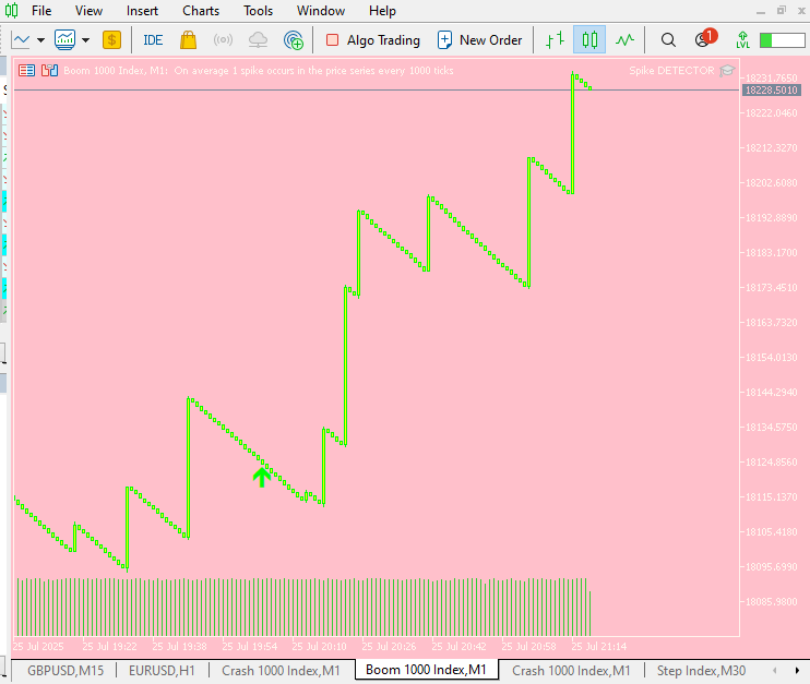
Here’s an earlier test run of the system. Occasionally, the EA will signal an entry—these “OPEN” instructions appear in the MetaTrader 5 logs, though no arrow is placed on the chart. Whether a visual marker appears depends on the signal’s strength.

MetaTrader 5 logs

2025.07.25 19:55:01.445 Spike DETECTOR (Boom 1000 Index,M1)     [SpikeEA] <<< HTTP 200 – {"Pbuy":0.999,"Psell":0.0,"scale_in":null
,"side":"BUY","signal":"OPEN","strength":1.0

MetaTrader 5 Chart

Conclusion

Bringing MQL5 and Python together has given us a powerful, flexible trading framework—one that leverages the best of both worlds. On the MQL5 side, our EA seamlessly captures spikes, MACD divergence, RSI, ATR, Kalman‑filtered slopes and Prophet deltas, then streams those metrics straight into Python. On the Python side, a single engine.py script (with collect, history, train, backtest, serve commands) handles the heavy lifting of model training and live serving. In our setup, we leaned on MQL5’s EA to supply all the necessary feature data, so we only ever needed to run:

python engine.py train
python engine.py serve

Skipping collect and history because our EA already maintains and provides the full dataset for us.

The result? Within moments of hitting Serve, our Gradient Boosting models return real‑time BUY/SELL/WAIT signals back to MetaTrader 5 in under 50 ms per bar—ready to be acted on by our EA’s order logic. Whether you’re just getting started on the MQL5 website’s rich library of documentation and community examples, or you’re an experienced quant looking to plug in new feature generators or algorithms, this end‑to‑end pipeline scales effortlessly across symbols and strategies.

Thank you to the MQL5 community and the wealth of code samples and forum insights available at mql5.com, your resources made this integration straightforward. I encourage everyone to explore further: tweak hyperparameters, add fresh indicators, or even containerize your Python server for production. Most importantly, share your findings back with the community so we can all continue to advance data‑driven algorithmic trading together.

Chart Projector	Analytical Comment	Analytics Master	Analytics Forecaster	Volatility Navigator	Mean Reversion Signal Reaper
Signal Pulse	Metrics Board	External Flow	VWAP	Heikin Ashi	FibVWAP
RSI DIVERGENCE	Parabolic Stop and Reverse (PSAR)	Quarters Drawer Script	Intrusion Detector	TrendLoom Tool	Quarters Board
ZigZag Analyzer	Correlation Pathfinder	Market Structure Flip Detector Tool	Correlation Dashboard	Currency Strength Meter	PAQ Analysis Tool
Dual EMA Fractal Breaker	Pin bar, Engulfing and RSI divergence	Liquidity Sweep	Opening Range Breakout Tool	Boom and Crash Interceptor	CCI Zer-Line EA
Candlestick Recognition	Candlestick Detection using TA-Lib	Candle Range Tool	MetaTrader 5 Data Ingestor	Model Training and Deployment