Neural Networks in Trading: A Parameter-Efficient Transformer with Segmented Attention (PSformer)

Introduction

Multivariate time series forecasting is an important task in deep learning, with practical applications in meteorology, energy, anomaly detection, and financial analysis. With the rapid advancement of artificial intelligence, significant efforts have been made to design innovative models that improve forecasting accuracy. Transformer-based architectures, in particular, have attracted considerable attention due to their proven effectiveness in natural language processing and computer vision. Moreover, large-scale, pre-trained Transformer models have demonstrated strong performance in time series forecasting, showing that increasing model parameters and training data can substantially enhance predictive capabilities.

At the same time, many simple linear models achieve competitive results compared to more complex Transformer-based architectures. Their success in time series forecasting is likely due to their lower complexity, which reduces the risk of overfitting to noisy or irrelevant data. Even with limited datasets, these models can effectively capture stable, reliable patterns.

To address the challenges of modeling long-term dependencies and capturing complex temporal relationships, the PatchTST approach processes data using patching techniques to extract local semantics, delivering strong performance. However, PatchTST uses channel-independent structures and has significant potential for further improvement in modeling efficiency. Furthermore, the unique nature of multivariate time series, where temporal and spatial dimensions differ significantly from other data types, offers many unexplored opportunities.

One way to reduce model complexity in deep learning is parameter sharing (PS), which significantly decreases the number of parameters while improving computational efficiency. In convolutional networks, filters share weights across spatial positions, extracting local features with fewer parameters. Similarly, LSTM models share weight matrices across time steps, managing memory and information flow. In natural language processing, parameter sharing has been extended to Transformers by reusing weights across layers, reducing redundancy without compromising performance.

In multitask learning, the Task-Adaptive Parameter Sharing (TAPS) method selectively fine-tunes task-specific layers, maximizing parameter sharing while enabling efficient learning with minimal task-specific adjustments. Research indicates that parameter sharing can reduce model size, improve generalization, and lower overfitting risk across diverse tasks.

The authors of "PSformer: Parameter-efficient Transformer with Segment Attention for Time Series Forecasting" propose an innovative Transformer-based model for multivariate time series forecasting that incorporates parameter sharing principles.

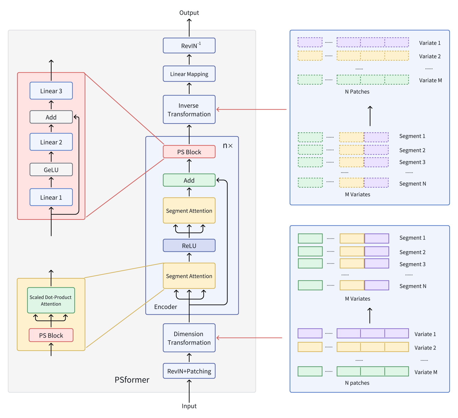
They introduce a Transformer encoder with a two-level segment-based attention mechanism, where each encoder layer includes a shared-parameter block. This block contains three fully connected layers with residual connections, enabling a low overall parameter count while maintaining effective information exchange across model components. To focus attention within segments, they apply a patching method that splits variable sequences into separate patches. Patches occupying the same position across different variables are then grouped into segments. Each segment becomes a spatial extension of a single-variable patch, effectively dividing the multivariate time series into multiple segments.

Within each segment, attention mechanisms enhance the capture of local spatio-temporal relationships, while cross-segment information integration improves overall forecasting accuracy. The authors also incorporate the SAM optimization method to further reduce overfitting without degrading learning performance. Extensive experiments on long-term time series forecasting datasets show that PSformer delivers strong results. PSformer outperforms state-of-the-art models in 6 out of 8 key forecasting benchmarks.

The PSformer Algorithm

A multivariate time series X ∈ RM×L contains M variables ans a look-back window of length L. The sequence length L is evenly divided into N non-overlapping patches of size P. Then, P(i) from the M variables forms the i-th segment, representing a cross-section of length C (where C=M×P).

The key components of PSformer are Segment Attention (SegAtt) and the Parameter-Sharing Block (PS). The PSformer encoder serves as the model's core, containing both the SegAtt module and the PS block. The PS block provides parameters for all encoder layers through parameter sharing.

As in other time series forecasting architectures, the PSformer authors use the RevIN method to effectively address distribution shift issues.

Segment spatio-temporal attention (SegAtt) merges patches from different channels at the same position into a segment and establishes spatio-temporal relationships across segments. Specifically, the original time series X ∈ RM×L is first divided into patches where L=P×N, then reshaped into X ∈ R(M×P)×N, by merging dimensions M and P. This produces X ∈ RC×N (where C=M×P), enabling cross-channel information fusion.

In this transformed space, the data is processed by two consecutive modules with identical architecture, separated by a ReLU activation. Each module contains a parameter-sharing block and a Self-Attention mechanism which is already familiar to us. While computing 𝑸uery ∈ RC×N, 𝑲ey ∈ RC×N and 𝑽alue ∈ RC×N matrices involves non-linear transformations of input Xin along segments into N-dimensional representations, the scaled dot-product attention primarily distributes focus across the entire C dimension. This allows the model to learn dependencies between spatio-temporal segments across both channels and time.

This mechanism integrates information from different segments by computing Q, K, and V. It also captures local spatio-temporal dependencies within each segment while also modeling long-term inter-segment relationships across extended time steps. The final output is Xout ∈ RC×N, completing the attention process.

PSformer introduces a new Parameter Shared Block (PS Block), consisting of three fully connected layers with residual connections. Specifically, it uses three learnable linear mappings Wj ∈ RN×N с j ∈ {1, 2, 3}. The outputs of the first two layers are computed as follows:

This structure is analogous to a FeedForward block with residual connections. The intermediate output 𝑿out then serves as the input for the third transformation:

Overall, the PS block can be expressed as:

The PS block stucture enables non-linear transformations while preserving the trajectory of a linear mapping. Although three layers in the PS block have different parameters, the entire PS block is reused across multiple positions in the PSformer encoder, ensuring that the same 𝑾S block parameters are common to all these positions. Specifically, the PS block's parameters are shared in three parts of each PSformer encoder: including the two SegAtt modules and the final PS block. This parameter-sharing strategy reduces the total parameter count while maintaining model expressiveness.

The two-stage SegAtt mechanism can be compared to a FeedForward block in a vanilla Transformer, where the MLP is replaced with attention operations. Residual connections are added between the input and output, and the result is passed to the final PS block.

A dimensional transformation is then applied to obtain 𝑿o⁢ut ∈ RM×L, where C=M×P and L=P×N.

After passing through n layers of PSformer, a final transformation is applied to project the output onto the forecasting horizon F.

where 𝑿pred ∈ RM×F and 𝑾F ∈ RL×F represent linear mapping.

The original visualization of the PSformer framework is provided below.

Implementation in MQL5

After covering the theoretical aspects of the PSformer framework, we now move on to the practical implementation of our vision of the proposed approaches using MQL5. Of particular interest to us is the algorithm for implementing the Parameter-Sharing Block (PS Block).

Parameter Shared Block

As noted earlier, in the authors' original implementation the PS Block consists of three fully connected layers whose parameters are applied to all analyzed segments. From our perspective, there's nothing complicated. We have repeatedly employed convolutional layers with non-overlapping analysis windows in similar situations. The real challenge lies elsewhere: in the mechanism for sharing parameters across multiple blocks.

On the one hand, we could certainly reuse the same block multiple times within a single layer. However, this introduces the problem of preserving data for the backpropagation pass. When an object is reused for multiple feed-forward passes, the result buffer will store new outputs, overwriting those from previous feed-forward passes. In a typical neural layer workflow, this is not an issue, since we consistently alternate between feed-forward and backpropagation passes. After each backward pass, the results from the preceding feed-forward pass are no longer needed and can safely be overwritten. But when this alternation is disrupted, we face the problem of retaining all the data required for a correct backpropagation pass.

In such cases, we must store not only the final outputs of the block, but also all intermediate values. Or we must recompute them, which increases the model's computational complexity. Additionally, a mechanism is needed to synchronize buffers at specific points to correctly compute the error gradient.

Clearly, implementing these requirements would require changes to our data exchange interfaces between neural layers. This, in turn, would trigger broader modifications to our library functionality.

The second option is to establish a mechanism for full-fledged sharing of a single parameter buffer among several identical neural layers. This approach, however, is not without its own "hidden pitfalls".

Recall that when we explored the Deep Deterministic Policy Gradient framework, we implemented a soft parameter update algorithm for the target model. Copying parameters after each update, however, is computationally expensive. Ideally, we would replace the parameter buffers in the relevant objects with shared parameter matrices.

Here, in addition to the parameter matrix itself, we must also share the momentum buffers used during parameter updates. Using separate momentum buffers at different stages can bias the parameter update vector toward one of the internal layers.

There is another critical point. Шn this implementation, parameters used in the backpropagation pass may differ from those used in the feed-forward pass. This may sound unusual, but let's illustrate it with a simple example involving two consecutive layers that share parameters. During the feed-forward pass, both layers use parameters W and produce outputs O1 and O2 respectively. At the gradient distribution stage, we compute error gradients G1 and G2 respectively. SO, the error gradient propagation process is correct. At this stage, the model parameters remain unchanged, and all error gradients correctly correspond to the feed-forward parameters W. However, if we update the parameters in one of the layers, for example, the second, we get adjusted parameters W'. We immediately encounter a mismatch: the error gradients no longer correspond to the updated parameters. Directly applying a mismatched gradient can distort the training process.

One solution to this problem is to determine the target values for a given layer based on the outputs from the last feed-forward pass and the corresponding error gradients, then perform a new feed-forward pass with the updated parameters to compute a corrected error gradient. If this sounds familiar, it is because this approach closely resembles the SAM optimization algorithm we discussed in previous articles. Indeed, by adding parameter updates before executing the repeated forward pass, we obtain the full SAM optimization procedure.

This is precisely why the authors of the PSformer framework recommend using SAM optimization. It allows us to tolerate the risk of gradient–parameter mismatches, since the gradients are recomputed before parameter updates. In other scenarios, however, such mismatches could pose a serious problem.

Considering all the above, we decided to adopt the second approach - sharing parameter buffers between identical layers.

As noted earlier, the PS Block in the original paper employs three fully connected layers, which we replace with convolutional layers. We therefore begin our parameter-sharing implementation with the CNeuronConvSAMOCL convolutional layer object.

In our convolutional parameter-sharing layer, we substitute only the pointers to the parameter and momentum buffers. All other buffers and internal variables must still match the dimensions of the parameter matrix. Naturally, this requires adjustments to the object's initialization method. Before doing so, we create two auxiliary methods: InitBufferLike and ReplaceBuffer.

InitBufferLike creates a new buffer filled with zero values based on a given reference buffer. Its algorithm is quite simple. It accepts two pointers to data buffer objects as parameters. First, it checks whether the reference buffer pointer (master) is valid. The presence of a valid reference pointer is critical for subsequent operations. If this check fails, the method terminates and returns false.

bool CNeuronConvSAMOCL::InitBufferLike(CBufferFloat *&buffer, CBufferFloat *master)
  {
   if(!master)
      return false;

If the first checkpoint is passed successfully, we check the relevance of the pointer to the created buffer. But here, if we get a negative result, we simply create a new instance of the object.

   if(!buffer)
     {
      buffer = new CBufferFloat();
      if(!buffer)
         return false;
     }

And don't forget to check if the new buffer has been created correctly.

Next, we initialize the buffer of the required size with zero values.

   if(!buffer.BufferInit(master.Total(), 0))
      return false;

Then we create its copy in the OpenCL context.

   if(!buffer.BufferCreate(master.GetOpenCL()))
      return false;
//---
   return true;
  }

The method then concludes by returning the logical result of the operation to the caller.

Second method ReplaceBuffer substitutes the pointer to the specified buffer. At first glance, we don't need a whole method to assign a pointer to an internal variable object. However, in the method body we check and, if necessary, remove excess data buffers. This allows us to use both RAM and OpenCL-context memory more efficiently.

void CNeuronConvSAMOCL::ReplaceBuffer(CBufferFloat *&buffer, CBufferFloat *master)
  {
   if(buffer==master)
     return;
   if(!!buffer)
     {
      buffer.BufferFree();
      delete buffer;
     }
//---
   buffer = master;
  }

After creating the auxiliary methods, we proceed to building a new initialization algorithm for the convolutional layer object based on a reference instance InitPS. In this method, instead of receiving a full set of constants defining the object architecture, we accept only a pointer to a reference object.

bool CNeuronConvSAMOCL::InitPS(CNeuronConvSAMOCL *master)
  {
   if(!master ||
      master.Type() != Type()
     )
      return false;

In the method body, we check if the received pointer is correct and the object types match.

Next, instead of build a whole set of parent class methods, we simply transfer the values of all inherited parameters from the reference object.

   alpha = master.alpha;
   iBatch = master.iBatch;
   t = master.t;
   m_myIndex = master.m_myIndex;
   activation = master.activation;
   optimization = master.optimization;
   iWindow = master.iWindow;
   iStep = master.iStep;
   iWindowOut = master.iWindowOut;
   iVariables = master.iVariables;
   bTrain = master.bTrain;
   fRho = master.fRho;

 Next, we create result and error gradient buffers similar to those in the reference object.

   if(!InitBufferLike(Output, master.Output))
      return false;
   if(!!master.getPrevOutput())
      if(!InitBufferLike(PrevOutput, master.getPrevOutput()))
         return false;
   if(!InitBufferLike(Gradient, master.Gradient))
      return false;

After that, we transfer the pointers first to the weight and moment buffers inherited from the basic fully connected layer.

   ReplaceBuffer(Weights, master.Weights);
   ReplaceBuffer(DeltaWeights, master.DeltaWeights);
   ReplaceBuffer(FirstMomentum, master.FirstMomentum);
   ReplaceBuffer(SecondMomentum, master.SecondMomentum);

We repeat a similar operation for the buffers of convolutional layer parameters and their moments.

   ReplaceBuffer(WeightsConv, master.WeightsConv);
   ReplaceBuffer(DeltaWeightsConv, master.DeltaWeightsConv);
   ReplaceBuffer(FirstMomentumConv, master.FirstMomentumConv);
   ReplaceBuffer(SecondMomentumConv, master.SecondMomentumConv);

Next, we need to create buffers of adjusted parameters. However, both adjusted parameter buffers may not be created under certain conditions. The buffer of adjusted parameters of a fully connected layer is created only if there are outgoing connections. Therefore, we first check the size of this buffer in the reference object. We create the relevant buffer only when necessary.

   if(master.cWeightsSAM.Total() > 0)
     {
      CBufferFloat *buf = GetPointer(cWeightsSAM);
      if(!InitBufferLike(buf, GetPointer(master.cWeightsSAM)))
         return false;
     }

Otherwise, we clear this buffer, reducing memory consumption.

   else
     {
      cWeightsSAM.BufferFree();
      cWeightsSAM.Clear();
     }

The buffer of adjusted parameters of incoming connections is created when the blur area coefficient is greater than 0.

   if(fRho > 0)
     {
      CBufferFloat *buf = GetPointer(cWeightsSAMConv);
      if(!InitBufferLike(buf, GetPointer(master.cWeightsSAMConv)))
         return false;
     }

Otherwise, we clear this buffer.

   else
     {
      cWeightsSAMConv.BufferFree();
      cWeightsSAMConv.Clear();
     }

Technically, instead of using the blur coefficient, we could check the size of the buffer containing the adjusted parameters of the incoming connections of the reference object - just as we do for the buffer of adjusted parameters for the outgoing connections. However, we know that if the blur coefficient is greater than zero, this buffer must exist. Thus, we include an additional control. If an attempt is made to create a zero-length buffer, the process will fail, throwing an error and halting initialization. This helps prevent more serious issues later in execution.

At the end of the initialization method, we transfer all objects into a single OpenCL context and return the logical result of the operation to the calling program.

   SetOpenCL(master.OpenCL);
//---
   return true;
  }

After modifying the convolutional layer object, we proceed to the next stage of our work. Now we will create the Parameter-Sharing Block (PS Block) itself. For this, we introduce a new object: CNeuronPSBlock. As outlined in the theoretical section, the PS Block consists of three sequential data transformation layers. Each has a square parameter matrix, ensuring that the input and output tensor dimensions remain consistent for both the block as a whole and its internal layers. Between the first two layers, a GELU activation function is applied. After the second layer, a residual connection is added to the original input.

To implement this architecture, the new object will contain two internal convolutional layers, while the final convolutional layer will be represented directly by the structure of our class itself, inheriting the base functionality from the convolutional layer class. Since we will be using SAM optimization during training, all convolutional layers in the architecture will be SAM-compatible. The structure of the new class is shown below.

class CNeuronPSBlock :  public CNeuronConvSAMOCL
  {
protected:
   CNeuronConvSAMOCL acConvolution[2];
   CNeuronBaseOCL    cResidual;
   //---
   virtual bool      feedForward(CNeuronBaseOCL *NeuronOCL);
   virtual bool      updateInputWeights(CNeuronBaseOCL *NeuronOCL);
   virtual bool      calcInputGradients(CNeuronBaseOCL *NeuronOCL);

public:
                     CNeuronPSBlock(void) {};
                    ~CNeuronPSBlock(void) {};
   //---
   virtual bool      Init(uint numOutputs, uint myIndex, COpenCLMy *open_cl, 
                          uint window, uint window_out, uint units_count, 
                          uint variables, float rho, 
                          ENUM_OPTIMIZATION optimization_type, uint batch);
   virtual bool      InitPS(CNeuronPSBlock *master);
   //---
   virtual int       Type(void)   const         {  return defNeuronPSBlock;   }
   //--- methods for working with files
   virtual bool      Save(int const file_handle);
   virtual bool      Load(int const file_handle);
   //---
   virtual CLayerDescription* GetLayerInfo(void);
   virtual void      SetOpenCL(COpenCLMy *obj);
  };

As seen in the structure, the new object declares two initialization methods. This is done on purpose. Init – the standard initialization method, where the architecture of the object is explicitly defined by the parameters passed to the method. InitPS – analogous to the method of the same name in the convolutional layer class, it creates a new object based on the structure of a reference object. During this process, pointers to parameter and momentum buffers are copied from the reference. Let's consider in more detail the algorithm for constructing the specified methods.

As mentioned above, the Init method receives a set of constants in its parameters, allowing the architecture of the object to be fully determined.

bool CNeuronPSBlock::Init(uint numOutputs, uint myIndex, COpenCLMy *open_cl,
                          uint window, uint window_out, uint units_count,
                          uint variables, float rho,
                          ENUM_OPTIMIZATION optimization_type, uint batch)
  {
   if(!CNeuronConvSAMOCL::Init(numOutputs, myIndex, open_cl, window, window, window_out,
                               units_count, variables, rho, optimization_type, batch))
      return false;

In the method body, we immediately forward all received parameters to the identically named method of the parent class. As you know, the parent method already contains the necessary parameter validation points and initialization logic for inherited objects.

Since all convolutional layers inside the PS Block have the same dimensions, the initialization of the first internal convolutional layer uses the exact same parameters.

   if(!acConvolution[0].Init(0, 0, OpenCL, iWindow, iWindow, iWindowOut, units_count,
                             iVariables, fRho, optimization, iBatch))
      return false;
   acConvolution[0].SetActivationFunction(GELU);

We then add the GELU activation function, as suggested by the PSformer authors.

However, we also allow the user to modify the tensor dimensions at the block output. Therefore, when initializing the second internal convolutional layer, which is followed by a residual connection, we swap the parameters for the analysis window size and the number of filters. This ensures that the output dimensions match those of the original input data.

   if(!acConvolution[1].Init(0, 1, OpenCL, iWindowOut, iWindowOut, iWindow, units_count,
                             iVariables, fRho, optimization, iBatch))
      return false;
   acConvolution[1].SetActivationFunction(None);

We do not use the activation function here.

Next, we add a base neural layer to store the residual connection data. Its size corresponds to the result buffer of the second nested convolutional layer.

   if(!cResidual.Init(0, 2, OpenCL, acConvolution[1].Neurons(), optimization, iBatch))
      return false;
   if(!cResidual.SetGradient(acConvolution[1].getGradient(), true))
      return false;
   cResidual.SetActivationFunction(None);

Immediately after creating the object based on the reference instance, we replace the error-gradient buffer. This optimization allows us to reduce the number of data-copy operations during the backpropagation pass.

Next, we explicitly disable the activation function for our parameter-sharing block and complete the method, returning a logical result to the caller.

   SetActivationFunction(None);
//---
   return true;
  }

The second initialization method is somewhat simpler. It receives a pointer to a reference object and directly passes it to the identically named method of the parent class.

It is important to note that the parameter types in the current method differ from those in the parent class. So, we explicitly specify the type of the object being passed.

bool CNeuronPSBlock::InitPS(CNeuronPSBlock *master)
  {
   if(!CNeuronConvSAMOCL::InitPS((CNeuronConvSAMOCL*)master))
      return false;

The parent class method already contains the necessary validation checks, as well as the logic for copying constants, creating new buffers, and storing pointers to the parameter and momentum buffers.

We then iterate through the internal convolutional layers, calling their corresponding initialization methods and copying data from the respective reference objects.

   for(int i = 0; i < 2; i++)
      if(!acConvolution[i].InitPS(master.acConvolution[i].AsObject()))
         return false;

The residual-connection layer does not contain trainable parameters, and its size matches the result buffer of the second internal convolutional layer. Therefore, its initialization logic is taken entirely from the main initialization method.

   if(!cResidual.Init(0, 2, OpenCL, acConvolution[1].Neurons(), optimization, iBatch))
      return false;
   if(!cResidual.SetGradient(acConvolution[1].getGradient(), true))
      return false;
   cResidual.SetActivationFunction(None);
//---
   return true;
  }

As before, we replace the pointers to the error-gradient buffer.

With the initialization methods complete, we move on to the feed-forward algorithms. This part is relatively straightforward. The method receives a pointer to the input data object, which we pass directly to the feed-forward method of the first internal convolutional layer.

bool CNeuronPSBlock::feedForward(CNeuronBaseOCL *NeuronOCL)
  {
   if(!acConvolution[0].FeedForward(NeuronOCL))
      return false;

The results are then passed sequentially to the next convolutional layer. Afterward, we sum the resulting values with the original input. W save the sum in the residual-connection buffer.

   if(!acConvolution[1].FeedForward(acConvolution[0].AsObject()))
      return false;
   if(!SumAndNormilize(NeuronOCL.getOutput(), acConvolution[1].getOutput(), cResidual.getOutput(),
                                                                       iWindow, true, 0, 0, 0, 1))
      return false;

Here, we diverge slightly from the original PSformer algorithm: we normalize the residual tensor before passing it to the final convolutional layer, whose functionality is inherited from the parent class.

   if(!CNeuronConvSAMOCL::feedForward(cResidual.AsObject()))
      return false;
//---
   return true;
  }

The method concludes by returning the logical result of the operation to the caller.

The error-gradient distribution method calcInputGradients is also simple but has important nuances. It receives a pointer to the source-data layer object, into which we must propagate the error gradient.

bool CNeuronPSBlock::calcInputGradients(CNeuronBaseOCL *NeuronOCL)
  {
   if(!NeuronOCL)
     return false;

First, we check the validity of the received pointer - if invalid, further processing is meaningless.

We then pass the gradients backward through all convolutional layers in reverse order.

   if(!CNeuronConvSAMOCL::calcInputGradients(cResidual.AsObject()))
      return false;
   if(!acConvolution[0].calcHiddenGradients(acConvolution[1].AsObject()))
      return false;
   if(!NeuronOCL.calcHiddenGradients(acConvolution[0].AsObject()))
      return false;

Note that no explicit error-gradient transfer is coded from the residual-connection object to the second internal convolutional layer. However, thanks to our earlier pointer substitution for data buffers, information is still transferred in full.

After sending the gradient back to the source-data layer through the convolutional layer pipeline, we also add the gradient from the residual-connection branch. There are two possible cases, depending on whether the source-data object has an activation function.

I want to remind you that we pass the error gradient to the residual connections object without adjusting for the derivative of the activation function. We explicitly indicated its absence for this object.

Therefore, given the absence of an activation function for the source data object, we only need to add the corresponding values of the two buffers.

   if(NeuronOCL.Activation() == None)
     {
      if(!SumAndNormilize(NeuronOCL.getGradient(), cResidual.getGradient(), NeuronOCL.getGradient(),
                                                                        iWindow, false, 0, 0, 0, 1))
         return false;
     }

Otherwise, we first adjust the obtained error gradient using the derivative of the activation function into a free buffer. And then, we sum the obtained results with those previously accumulated in the source-data object buffer.

   else
     {
      if(!DeActivation(NeuronOCL.getOutput(), cResidual.getGradient(), cResidual.getPrevOutput(), 
                                                                           NeuronOCL.Activation()) ||
         !SumAndNormilize(NeuronOCL.getGradient(), cResidual.getPrevOutput(), NeuronOCL.getGradient(),
                                                                          iWindow, false, 0, 0, 0, 1))
         return false;
     }
//---
   return true;
  }

Then we complete the method.

A few words should be said about the updateInputWeights method where we update block parameters. This block is straightforward – we just call the corresponding methods in the parent class and in the internal objects containing trainable parameters.

bool CNeuronPSBlock::updateInputWeights(CNeuronBaseOCL *NeuronOCL)
  {
   if(!CNeuronConvSAMOCL::updateInputWeights(cResidual.AsObject()))
      return false;
   if(!acConvolution[1].UpdateInputWeights(acConvolution[0].AsObject()))
      return false;
   if(!acConvolution[0].UpdateInputWeights(NeuronOCL))
      return false;
//---
   return true;
  }

However, using SAM optimization imposes strict requirements on the order of operations. During SAM optimization, we perform a second forward pass with adjusted parameters. This updates the result buffer While this is harmless for updating the current layer parameters, it can disrupt parameter updates in subsequent layers. This is because they use the previous layer's feed-forward results. To prevent this, we must update parameters in reverse order through the internal objects. This will ensure each layer's parameters are adjusted before its input buffer is altered by another layer.

This concludes our discussion of the CNeuronPSBlock parameter sharing block algorithms. The full source code for this class and its methods can be found in the provided attachment.

Our work is not yet complete, but the article turned out to be long. Therefore, we will take a short break and continue the work in the next article.

Conclusion

In this article, we explored the PSformer framework, whose authors emphasize its high accuracy in time series forecasting and efficient use of computational resources. The PSformer's key architectural components include the Parameter-Sharing Block (PS) and Segment-Based Spatio-Temporal Attention (SegAtt). They allow for effective modeling of both local and global time series dependencies while reducing parameter count without sacrificing forecast quality.

In the practical section, we began implementing our own interpretation of the proposed methods in MQL5. Our work is not yet complete. In the next article, we will continue development and evaluate the effectiveness of these approaches on real historical datasets relevant to our specific tasks.

References

PSformer: Parameter-efficient Transformer with Segment Attention for Time Series Forecasting

Other articles from this series

Programs used in the article

#	Name	Type	Description
1	Research.mq5	Expert Advisor	Expert Advisor for collecting examples
2	ResearchRealORL.mq5	Expert Advisor	Expert Advisor for collecting examples using the Real-ORL method
3	Study.mq5	Expert Advisor	Model training Expert Advisor
4	StudyEncoder.mq5	Expert Advisor	Encoder training Expert Advisor
5	Test.mq5	Expert Advisor	Model testing Expert Advisor
6	Trajectory.mqh	Class library	System state description structure
7	NeuroNet.mqh	Class library	A library of classes for creating a neural network
8	NeuroNet.cl	Library	OpenCL program code library