Price Action Analysis Toolkit Development (Part 41): Building a Statistical Price-Level EA in MQL5

Contents

• Introduction
• Strategy Logic
• Code Breakdown
• Outcomes
• Conclusion

Introduction

Statistics has always been central to financial analysis because it turns noisy market data into measurable, comparable quantities. In this installment of the Price Action Analysis Toolkit, we apply those same statistical tools directly to candlesticks: instead of treating each bar as a single click of information, we compress many bars into reproducible price levels and distributional features that make the market’s recent behavior interpretable.

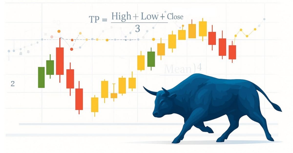
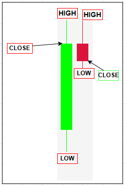
Every candle can be summarized by a typical price, defined here as the arithmetic average of its three main components:

Using TP to derive mean, median, mode; and percentile levels is therefore essential: the mode highlights the price cluster where the market spends the most time and often maps to practical support or resistance; the median identifies the robust center of the distribution and reveals directional shifts when price crosses it; the mean (and derived z-score) provides a balance point sensitive to large moves and is useful for volatility-normalized signals; finally, percentiles (P25/P75) frame the middle 50% of price action (IQR) and help distinguish tight consolidation from broad dispersion. In short, TP-based statistics produce reference levels that are both statistically meaningful and directly relevant to intraday price behavior.

In this article we show how those metrics translate into practical, chart-friendly signals: they become horizontal reference lines (mean, median, P25/P75, modal levels), inputs to ATR-scaled thresholds that distinguish breakouts from reversals, and the basis for a z-score signal engine that flags unusually extreme price action. Crucially, the implementation we present (the KDE Level Sentinel EA) emphasizes reproducibility and usability: snapshots freeze reference levels for forward monitoring, labels are kept stable and non-overlapping, and signals are drawn as precise chart arrows that mark the exact triggering price.

Read on to learn the math behind each metric, the implementation details in MQL5, and how to interpret the EA’s outputs so you can move from raw candlesticks to clear, testable trading hypotheses.

Strategy Logic

Like I mentioned, we are trying to implement statistical methods to price action, so we are using typical price for all statistical calculations. Typical Price (TP) is calculated by adding a bar’s high, low, and close and dividing the sum by three; it balances the trading range with the closing level, smoothing isolated spikes and producing a steadier series than the close alone. By incorporating intra-bar extremes without requiring the open, TP provides richer inputs for distributional statistics—mean, median, and kernel density estimates—improving stability and signal quality for downstream models. Compared with alternatives such as Close, HL/2, or OHLC4, TP strikes a pragmatic middle ground: it captures both range and direction in a compact, robust input ideal for price-action statistical analysis.

Below are the statistical metrics we derive from the typical price (TP). Each metric highlights a different aspect of how price behaves over time—from central tendency and dispersion to frequency and structure. 

Metrics derived from TP:

• Mean (Average)
• Median
• Mode
• Standard Deviation
• Variance
• Range (High–Low Spread)
• Skewness & Kurtosis (optional advanced)

Let's examine them one by one so that we can see how raw candlestick data transforms into meaningful price levels and signals that guide price action analysis.

1. Mean (Average)

The mean represents the central value of all typical prices within a sample. Although it is sensitive to extreme spikes, it offers a reliable overview of where prices tend to hover on average. For instance, if a person earns $1000, $1200, and $1100 in three months, the mean salary is (1000+1200+1100)/3=1100, reflecting the overall income level. Likewise, in trading, the mean TP highlights the average price around which the market fluctuates.

MQL5 Implementation:

double Mean(const double &values[])
{
   double sum = 0.0;
   for(int i=0; i<ArraySize(values); i++)
      sum += values[i];
   return sum / ArraySize(values);
}

2. Median

The median is the middle value in an ordered set of typical prices. Unlike the mean, it is unaffected by extreme highs or lows, making it a robust measure of central tendency. For example, given test scores of 50, 55, 60, 95, and 100, the median is 60, representing the true midpoint of performance. In trading, the median TP shows the balanced center of price action without distortion from unusual spikes.

MQL5 Implementation:

double Median(double &values[])
{
   ArraySort(values, WHOLE_ARRAY, 0, MODE_ASCEND);
   int size = ArraySize(values);
   if(size % 2 == 0)
      return (values[size/2 - 1] + values[size/2]) / 2.0;
   else
      return values[size/2];
}

3. Mode

The mode identifies the most frequently occurring value in a dataset, offering insight into natural clustering. For example, in a group where shoe sizes are 7, 8, 8, 9, 8, 7, 10, 8, 9, and 7, the most common size is 8—the mode. Similarly, in trading, the mode of TP points to price levels where the market spends the most time, often aligning with strong support or resistance zones.

MQL5 Implementation:

double Mode(const double &values[])
{
   double mode = values[0];
   int maxCount = 0;

   for(int i=0; i<ArraySize(values); i++)
   {
      int count = 0;
      for(int j=0; j<ArraySize(values); j++)
      {
         if(values[j] == values[i]) count++;
      }
      if(count > maxCount)
      {
         maxCount = count;
         mode = values[i];
      }
   }
   return mode;
}

4. Standard Deviation

Standard deviation measures how far values deviate from the mean, capturing the degree of variability. Consider two people with the same average daily steps: one logs 7900, 8000, and 8100 steps, while the other logs 2000, 15,000, and 5000. Both average around 8000, but the second has far greater variation. Applied to trading, standard deviation of TP distinguishes calm, steady markets from volatile, unstable ones.

MQL5 Implementation:

double StandardDeviation(const double &values[])
{
   double mean = Mean(values);
   double sum = 0.0;
   for(int i=0; i<ArraySize(values); i++)
      sum += MathPow(values[i] - mean, 2);
   return MathSqrt(sum / ArraySize(values));
}

5. Variance

Variance is the square of standard deviation and quantifies the spread of values around the mean in squared units. While less intuitive than standard deviation, it magnifies large deviations and provides a consistent basis for comparing volatility across instruments. In the context of TP, variance highlights how widely price levels disperse, offering another lens on market stability.

MQL5 Implementation:

double Variance(const double &values[])
{
   double mean = Mean(values);
   double sum = 0.0;
   for(int i=0; i<ArraySize(values); i++)
      sum += MathPow(values[i] - mean, 2);
   return sum / ArraySize(values);
}

6. Range

The range captures the difference between the highest and lowest values in a dataset. For example, if weekly temperatures vary between 20°C and 35°C, the range is 15°C. In trading, the range of TP shows the breadth of market movement, helping traders quickly distinguish between tight consolidations and wide swings.

MQL5 Implementation:

double Range(const double &values[])
{
   double minVal = values[ArrayMinimum(values)];
   double maxVal = values[ArrayMaximum(values)];
   return maxVal - minVal;
}

7. Skewness or Kurtosis

Skewness measures the asymmetry of a distribution.

double Skewness(const double &values[])
{
   int n = ArraySize(values);
   double mean = Mean(values);
   double sd   = StandardDeviation(values);

   double sum = 0.0;
   for(int i=0; i<n; i++)
      sum += MathPow((values[i] - mean)/sd, 3);

   return (double)n / ((n-1)*(n-2)) * sum;
}

In a company where most employees earn $3000 but the CEO earns $50,000, the average salary is pulled upward, creating positive skew. Similarly, skewness in TP reveals whether prices have been more biased toward upward or downward extremes, signaling directional imbalances in market structure.

Kurtosis evaluates the “tailedness” of a distribution, or the likelihood of extreme outcomes. On a highway, if most cars travel between 60 and 70 km/h, kurtosis is low. If cars usually travel at that range but occasionally crawl at 20 or surge to 150, kurtosis is high.

double Kurtosis(const double &values[])
{
   int n = ArraySize(values);
   double mean = Mean(values);
   double sd   = StandardDeviation(values);

   double sum = 0.0;
   for(int i=0; i<n; i++)
      sum += MathPow((values[i] - mean)/sd, 4);

   return ((double)n*(n+1) / ((n-1)*(n-2)*(n-3))) * sum
          - (3.0*MathPow(n-1,2) / ((n-2)*(n-3)));
}

In trading, high kurtosis of TP indicates markets that are calm most of the time but prone to sudden, dramatic moves.

8. Percentiles (P25 and P75)

Percentiles divide the dataset into ranked positions, allowing us to understand where values fall within the distribution. The 25th percentile (P25) marks the point below which 25% of the typical prices lie, while the 75th percentile (P75) marks the level below which 75% of prices fall. Together, these two values form the interquartile range (IQR), which represents the middle 50% of all observations.

double p25 = Percentile(values, 0.25);
double p75 = Percentile(values, 0.75);

Print("P25 = ", DoubleToString(p25, _Digits), 
      " | P75 = ", DoubleToString(p75, _Digits));

In trading terms, P25 highlights the “lower cluster” of price activity, often showing where buyers are consistently stepping in, while P75 highlights the “upper cluster,” where sellers tend to dominate. When combined, these boundaries give us a more refined understanding of market concentration than mean or median alone. A tight IQR suggests consolidation, while a wide IQR suggests greater market dispersion.

The signal generation logic relies on the z-score of the most recent typical price, calculated as (TP – mean) / stddev using the current statistical window. When this standardized deviation moves beyond the configured entry threshold (ZScoreSignalEnter), the EA generates a long signal if the price is sufficiently below the mean (negative z-score) or a short signal if it is sufficiently above (positive z-score). Signals are only confirmed if the corresponding AllowLongSignals or AllowShortSignals settings are enabled. Once in a signal state, the EA waits until the z-score falls back within the defined exit band (ZScoreSignalExit) before clearing the signal and potentially alerting a reversal. Each signal transition triggers EmitAlertWithArrow, which draws a directional arrow on the chart and, depending on user settings, can also fire a pop-up alert, sound, or push notification.

Code Breakdown

This section describes the implementation details of KDE Level Sentinel.mq5, focusing on architecture, data flow, core algorithms, and the important helper routines that support chart visuals and level monitoring. The presentation is organized to help readers map the conceptual design to the corresponding code sections and configuration options.

Configuration and initialization

All user-configurable options are declared at the top of the source as input parameters. These include the analysis window (Lookback), whether to exclude the current forming bar; KDE and histogram settings (ModeBins, KDEGridPoints, KDEBandwidthFactor); z-score thresholds for signals; snapshot and monitoring controls (AutoSnapshotLevels, MonitorBars, TouchTolerancePips, BreakoutPips, ReversalPips, UseATRforThresholds), and UI/cleanup timing (TimerIntervalSeconds, CleanupIntervalSeconds). This single section acts as the EA’s control panel; changing an input alters the EA’s statistical lens and monitoring behavior without modifying the code.

// ---------- user inputs (control panel) ----------
input int    Lookback               = 1000;
input bool   ExcludeCurrent         = true;
input bool   UseWeightedByVol       = true;
input int    ModeBins               = 30;
input int    KDEGridPoints          = 100;
input double KDEBandwidthFactor     = 1.0;
input bool   DrawHistogramOnChart   = false;
input int    RefreshEveryXTicks     = 1;
input double ZScoreSignalEnter      = 2.0;
input double ZScoreSignalExit       = 0.8;
input bool   AutoSnapshotLevels     = true;
input int    MonitorBars            = 20;
input double TouchTolerancePips     = 3.0;
input bool   UseATRforThresholds    = true;
input double ATRMultiplier          = 0.5;
input int    ATRperiod              = 14;
input int    TimerIntervalSeconds   = 60;
input int    CleanupIntervalSeconds = 3600;

// ---------- OnInit (build names, cleanup, placeholders, start timer) ----------
int OnInit()
  {
   S_base = StringFormat("CSTATS_%s_%d", _Symbol, (int)TF);
   S_mean = S_base + "_MEAN";
   S_p25  = S_base + "_P25";
   // remove leftovers from previous runs
   RemoveExistingEAObjects();
   // create panel + placeholder HLINEs
   CreatePanel();
   CreateHLine(S_mean, 0.0, clrBlack, 2);
   CreateHLine(S_p25,  0.0, clrTeal,  1);
   // optionally clear previous snapshot
   if(ClearSnapshotOnStart) ClearSnapshot();
   // start periodic timer for housekeeping
   EventSetTimer(TimerIntervalSeconds);
   return(INIT_SUCCEEDED);
  }

During OnInit, the EA constructs canonical object and global variable name prefixes using S_base = StringFormat("CSTATS_%s_%d", _Symbol, (int)TF). This deterministic naming insulates multiple chart instances from accidental collisions and centralizes cleanup. Initialization proceeds to remove leftover objects from earlier instances, create a compact corner panel (summary labels), place placeholder horizontal lines for each core statistic (mean, ±SD, P25/P75, median, both modes), optionally clear prior snapshots, and start a periodic timer for housekeeping.

Data acquisition and main loop

The main computation occurs in OnTick, throttled by RefreshEveryXTicks to avoid excessive CPU use on high-frequency ticks. The routine copies Lookback bars from the configured timeframe into rates[] via CopyRates, using start = ExcludeCurrent ? 1 : 0 to optionally omit the forming candle. From rates[] it computes arrays of typical prices vals[] = (high + low + close) / 3.0 and tick volumes vols[] (when volume-weighting is enabled).

void OnTick()
  {
   tick_count++;
   if(tick_count < RefreshEveryXTicks) return;
   tick_count = 0;

   int start = ExcludeCurrent ? 1 : 0;
   int needed = Lookback;
   if(Bars(_Symbol, TF) - start < needed) return;

   MqlRates rates[];
   int copied = CopyRates(_Symbol, TF, start, needed, rates);
   if(copied <= 0) { Print("CopyRates failed: ", GetLastError()); return; }

   double vals[], vols[];
   ArrayResize(vals, copied);
   ArrayResize(vols, copied);
   for(int i = 0; i < copied; i++)
     {
      vals[i] = (rates[i].high + rates[i].low + rates[i].close) / 3.0; // typical price
      vols[i] = (double)rates[i].tick_volume;
     }

   // pass vals/vols into statistics routines...
  }

Statistical computation follows immediately: arithmetic mean, optional volume-weighted mean, sample variance and standard deviation, median, 25th/75th percentiles, a binned mode (ModeBinned) and a KDE-based mode (ModeKDE). The KDE bandwidth uses a Silverman-like rule h = 1.06 * sd * n^-0.2 scaled by KDEBandwidthFactor, then evaluates density on a uniform grid of KDEGridPoints and returns the grid point of greatest estimated density. The most recent typical price (latest) is used to compute a z-score (latest - mean) / stddev, which drives simple z-score entry/exit signals.
Computed statistics are published to horizontal lines and textual labels on the chart, and exported as global variables with keys prefixed by S_base to enable interoperable reads by other scripts or indicators.

Snapshotting and reference-level monitoring

When AutoSnapshotLevels is enabled the EA locks a single snapshot—persisting the current level estimates (mean, mean±sd, P25, P75, median, modes) and creating a refLevels[] array composed of RefLevel structs. Each RefLevel holds name, price, touched, touchTime, monitorLeft, highest, lowest, result (0 unknown, 1 breakout, -1 reversal, 2 no-follow), and resolvedTime. Snapshot HLINEs are named S_base + "_REF_" + name and either update canonical TXT objects (when a canonical label exists) or use REF-specific labels.

// take snapshot (single-shot)
void SnapshotReferenceLevels(double mean_val, double p25, double p75, double median_val, double mode_b, double mode_k)
  {
   snapshot_mean = mean_val;
   snapshot_p25  = p25;
   snapshot_p75  = p75;
   snapshot_median= median_val;
   // build refLevels
   ArrayResize(refLevels, 6);
   refLevels[0].name = "MEAN"; refLevels[0].price = snapshot_mean; refLevels[0].touched=false; refLevels[0].result=0;
   // ... fill others ...
   refSnapshotTaken = true;
   snapshotTakenTime = TimeCurrent();
  }

// monitor reference levels (called from OnTick)
void MonitorReferenceLevels(const MqlRates &rates[], int copied)
  {
   if(!refSnapshotTaken || copied <= 0) return;
   double barHigh = rates[0].high;
   double barLow  = rates[0].low;
   double barClose= rates[0].close;
   double pipPoints = pipToPointMultiplier();
   double touchTol = TouchTolerancePips * pipPoints;
   // compute thresholds (fixed or ATR-scaled)
   double breakoutThreshold = BreakoutPips * pipPoints;
   if(UseATRforThresholds)
     {
      int hATR = iATR(_Symbol, TF, ATRperiod);
      double atrBuf[];
      CopyBuffer(hATR,0,0,1,atrBuf);
      IndicatorRelease(hATR);
      breakoutThreshold = atrBuf[0] * ATRMultiplier;
     }

   for(int i=0;i<ArraySize(refLevels);i++)
     {
      RefLevel L = refLevels[i];
      if(L.result != 0) continue;
      if(!L.touched)
        {
         if(barHigh >= L.price - touchTol && barLow <= L.price + touchTol)
           {
            L.touched = true;
            L.touchTime = rates[0].time;
            L.monitorLeft = MonitorBars;
            L.highest = barHigh; L.lowest = barLow;
            refLevels[i] = L;
           }
        }
      else
        {
         // update highest/lowest and evaluate breakout/reversal
         if(barHigh > L.highest) L.highest = barHigh;
         if(barLow  < L.lowest)  L.lowest  = barLow;
         bool breakout = (L.highest >= L.price + breakoutThreshold);
         bool reversal = (L.lowest  <= L.price - breakoutThreshold);
         if(breakout && !reversal) { L.result = 1; L.resolvedTime = rates[0].time; DrawOutcome(L, true); }
         else if(reversal && !breakout) { L.result = -1; L.resolvedTime = rates[0].time; DrawOutcome(L, false); }
         else { if(--L.monitorLeft <= 0) { L.result = 2; L.resolvedTime = rates[0].time; DrawOutcome(L, false); } }
         refLevels[i] = L;
        }
     }
  }

Monitoring is implemented in MonitorReferenceLevels. For each unresolved reference, the latest bar’s high/low/close are compared against a touch tolerance (TouchTolerancePips converted to price units by pipToPointMultiplier()). A touch sets monitorLeft = MonitorBars and records the initial high/low. During the monitoring window the EA tracks the highest and lowest prices and evaluates breakout/reversal conditions. Thresholds are either fixed pip values or derived from ATR when UseATRforThresholds is true; ATR is obtained via iATR + CopyBuffer and scaled by ATRMultiplier to produce adaptive thresholds. An optional confirmation by bar close (UseCloseForConfirm) is supported. Outcomes are finalized either immediately on confirmation or at the end of the monitor window by comparing the observed extremes to the thresholds; they are then recorded and drawn via DrawOutcome.

Visuals and label placement

The EA prioritizes stable, non-overlapping chart annotations. Horizontal lines for statistics and snapshot references use CreateHLine, which updates existing objects if present and sets a metadata timestamp. Text labels are handled by CreateOrUpdateLineText, a placement routine that:

void CreateOrUpdateLineText(string name, datetime t, double price, string text)
  {
   long chart_id = ChartID();
   int x0 = 0, y0 = 0;
   bool ok = ChartTimePriceToXY(chart_id, 0, t, price, x0, y0);
   int fontSize = 10;
   int pixelThresh = MathMax(18, fontSize * 2);

   // collect used Y positions from existing OBJ_TEXT objects
   int usedYPositions[];
   ArrayResize(usedYPositions,0);
   int total = ObjectsTotal(0);
   for(int oi=0; oi<total; oi++)
     {
      string oname = ObjectName(0, oi);
      if(oname == name) continue;
      if(ObjectGetInteger(0, oname, OBJPROP_TYPE) != OBJ_TEXT) continue;
      long ot = (long)ObjectGetInteger(0, oname, OBJPROP_TIME);
      double op = ObjectGetDouble(0, oname, OBJPROP_PRICE);
      int xp=0, yp=0;
      if(ChartTimePriceToXY(chart_id,0,(datetime)ot,op,xp,yp))
        {
         ArrayResize(usedYPositions, ArraySize(usedYPositions)+1);
         usedYPositions[ArraySize(usedYPositions)-1] = yp;
        }
     }

   // attempt to find free Y slot
   int chosenY = y0;
   if(!IsYFree(chosenY, usedYPositions, pixelThresh))
     {
      int step = pixelThresh;
      bool found = false;
      for(int s=1; s<=20 && !found; s++)
        {
         int yUp = y0 - s*step;
         if(yUp >= 0 && IsYFree(yUp, usedYPositions, pixelThresh)) { chosenY = yUp; found = true; break; }
         int yDn = y0 + s*step;
         if(IsYFree(yDn, usedYPositions, pixelThresh)) { chosenY = yDn; found = true; break; }
        }
     }

   // convert chosen XY back to time/price; fallback if needed
   datetime tt = t; double pp = price;
   if(!ChartXYToTimePrice(chart_id, 0, x0, chosenY, tt, pp))
     { // fallback: nudge price slightly
      double point = SymbolInfoDouble(_Symbol, SYMBOL_POINT);
      int slotDelta = (chosenY - y0) / pixelThresh;
      pp = price + slotDelta * pixelThresh * point;
     }

   // create or update the OBJ_TEXT
   KeepSingleTextLabel(name);
   if(ObjectFind(0, name) >= 0)
     {
      ObjectSetInteger(0, name, OBJPROP_TIME, (long)tt);
      ObjectSetDouble(0, name, OBJPROP_PRICE, pp);
      ObjectSetString(0, name, OBJPROP_TEXT, text);
     }
   else
     {
      ObjectCreate(0, name, OBJ_TEXT, 0, tt, pp);
      ObjectSetString(0, name, OBJPROP_TEXT, text);
     }
   SetObjTimestamp(name);
  }

Attempts to map the target time+price to screen coordinates via ChartTimePriceToXY.

Gathers Y pixel positions of existing OBJ_TEXT objects (and canonical stat TXT peers) so that new labels avoid collisions.

Searches up/down in pixel steps (derived from font size) to locate a free slot (IsYFree) and converts the chosen XY slot back to time+price with ChartXYToTimePrice. If conversions fail, a robust fallback modifies position approximate to avoid crashes.

Enforces one _TXT object per HLINE using KeepSingleTextLabel.

This approach produces readable labels with minimal jitter during chart scrolling or resizing. Signal and outcome arrows are drawn by DrawArrowAt, which also creates a thin, exact HLINE at the arrow price to preserve precise alignment.

Histogram and KDE

DrawHistogram computes a frequency histogram of typical prices across ModeBins, draws HLINEs at bin centers with width proportional to count and creates compact count labels. ModeBinned computes a fast modal estimate by returning the center of the most populated bin. ModeKDE provides a smoother modal estimate by performing a naive kernel density estimate across a user-specified grid; its computational complexity is O(n × gridPts) and thus should be tuned for the chosen Lookback and intrabar rate.

// histogram drawing (bin counts => HLINE widths)
void DrawHistogram(const double &arr[], int n, int bins, int maxWidth)
  {
   double minv = ArrayMin(arr, n);
   double maxv = ArrayMax(arr, n);
   double binw = (maxv - minv) / bins;
   int counts[]; ArrayResize(counts, bins); ArrayInitialize(counts,0);
   for(int i=0;i<n;i++)
     {
      int b = (int)MathFloor((arr[i]-minv)/binw);
      if(b < 0) b=0; if(b >= bins) b=bins-1;
      counts[b]++;
     }
   // draw HLINE per bin with width proportional to counts[b]
  }

// KDE-based modal estimate
double ModeKDE(const double &a[], int n, int gridPts, double bwFactor)
  {
   double mn = ArrayMin(a,n), mx = ArrayMax(a,n);
   double sd = MathSqrt(Variance(a, n, false));
   double h = 1.06 * sd * MathPow((double)n, -0.2);
   if(h <= 0) h = (mx - mn) / 20.0;
   h *= bwFactor;
   double bestX = mn, bestD = -1.0;
   const double SQRT2PI = 2.5066282746310002;
   for(int g=0; g<gridPts; g++)
     {
      double x = mn + (double)g/(gridPts-1) * (mx - mn);
      double s = 0.0;
      for(int i=0;i<n;i++)
        {
         double u = (x - a[i]) / h;
         s += MathExp(-0.5 * u * u);
        }
      double dens = s / (n * h * SQRT2PI);
      if(dens > bestD) { bestD = dens; bestX = x; }
     }
   return(bestX);
  }

Metadata and lifecycle management

Every created chart object is associated with a metadata timestamp stored in a global variable keyed S_base + "_META_" + objectName via SetObjTimestamp. This enables RemoveOldObjects (invoked in OnTimer) to scan a list of candidate objects and delete those older than CleanupIntervalSeconds, preventing visual clutter on long-running charts. RemoveExistingEAObjects and CleanupAllMetaGlobals support controlled initialization and teardown by removing prior objects and their metadata.

// store timestamp meta
void SetObjTimestamp(string name)
  {
   string g = S_base + "_META_" + name;
   GlobalVariableSet(g, (double)TimeCurrent());
  }

// read meta timestamp
datetime GetObjTimestamp(string name)
  {
   string g = S_base + "_META_" + name;
   if(GlobalVariableCheck(g)) return (datetime)GlobalVariableGet(g);
   return 0;
  }

// remove objects older than ageSec
void RemoveOldObjects(int ageSec)
  {
   datetime now = TimeCurrent();
   string candidates[] = { S_mean, S_mean + "_TXT", S_p25, S_p25 + "_TXT", S_panel /* ... */ };
   for(int j=0;j<ArraySize(candidates);j++)
     {
      string nm = candidates[j];
      datetime ts = GetObjTimestamp(nm);
      if(ts == 0) continue;
      if((int)(now - ts) >= ageSec)
        {
         if(ObjectFind(0, nm) >= 0) ObjectDelete(0, nm);
         string g = S_base + "_META_" + nm;
         if(GlobalVariableCheck(g)) GlobalVariableDel(g);
        }
     }
  }

Alerts and signal handling

Z-score signals are evaluated each tick and subject to AllowLongSignals / AllowShortSignals. Enter thresholds are ZScoreSignalEnter and exit thresholds ZScoreSignalExit. On a signal state change, EmitAlertWithArrow draws the chart arrow and optionally triggers platform alerts (Alert()), sounds (PlaySound()), and push notifications (SendNotification()), while removing opposing signal arrows to limit chart noise.

// z-score signal logic (called from OnTick after stats computed)
int newSig = currentSignal;
if(zscore >= ZScoreSignalEnter && AllowLongSignals) newSig = 1;
else if(zscore <= -ZScoreSignalEnter && AllowShortSignals) newSig = -1;
else if(currentSignal == 1 && zscore < ZScoreSignalExit) newSig = 0;
else if(currentSignal == -1 && zscore > -ZScoreSignalExit) newSig = 0;

if(newSig != currentSignal)
  {
   if(newSig == 1)
     EmitAlertWithArrow("CSTATS LONG " + _Symbol + " z=" + DoubleToString(zscore,3), t_now, latest, true, S_arrow_long);
   else if(newSig == -1)
     EmitAlertWithArrow("CSTATS SHORT " + _Symbol + " z=" + DoubleToString(zscore,3), t_now, latest, false, S_arrow_short);
   else // clear arrows on exit
     {
      if(ObjectFind(0, S_arrow_long) >= 0) ObjectDelete(0, S_arrow_long);
      if(ObjectFind(0, S_arrow_short) >= 0) ObjectDelete(0, S_arrow_short);
     }
   currentSignal = newSig;
  }

// emit alert helper
void EmitAlertWithArrow(string message, datetime when, double price, bool isBuy, string arrowName)
  {
   DrawArrowAt(arrowName, when, price, isBuy);
   if(SendAlertOnSignal) Alert(message);
   if(PlaySoundOnSignal) PlaySound(SoundFileOnSignal);
   if(SendPushOnSignal) SendNotification(message);
  }

Statistical helpers and numerical considerations

The code implements standard array-based statistics; mean, weighted mean, sample variance, median (including even-n averaging), and linear-interpolated percentile—tailored to MQL5 array semantics. Auxiliary routines compute skewness and kurtosis if required for extension. Practically, KDE resolution (KDEGridPoints) and bandwidth (KDEBandwidthFactor) should be selected to balance smoothness, accuracy and CPU cost. ATR handle creation and release is performed per evaluation; for high-frequency execution, reusing indicator handles or computing ATR on new-bar only is recommended to reduce overhead.

double Mean(const double &a[], int n)
  {
   if(n<=0) return 0.0;
   double s=0.0;
   for(int i=0;i<n;i++) s += a[i];
   return s / n;
  }

double WeightedMean(const double &a[], const double &w[], int n)
  {
   if(n<=0) return 0.0;
   double sw=0.0, s=0.0;
   for(int i=0;i<n;i++) { s += a[i] * w[i]; sw += w[i]; }
   if(sw == 0.0) return Mean(a, n);
   return s / sw;
  }

double Variance(const double &a[], int n, bool sample)
  {
   if(n <= 1) return 0.0;
   double mu = Mean(a,n), s = 0.0;
   for(int i=0;i<n;i++) { double d = a[i] - mu; s += d * d; }
   return sample ? s / (n-1) : s / n;
  }

double Median(const double &a[], int n)
  {
   if(n <= 0) return 0.0;
   double tmp[]; ArrayResize(tmp, n); ArrayCopy(tmp, a); ArraySort(tmp);
   if((n % 2) == 1) return tmp[n/2];
   return (tmp[n/2 - 1] + tmp[n/2]) / 2.0;
  }

double Percentile(const double &a[], int n, double q)
  {
   if(n <= 0) return 0.0;
   double tmp[]; ArrayResize(tmp, n); ArrayCopy(tmp, a); ArraySort(tmp);
   if(q <= 0.0) return tmp[0];
   if(q >= 1.0) return tmp[n-1];
   double idx = q * (n - 1);
   int i0 = (int)MathFloor(idx); double frac = idx - i0;
   if(i0 + 1 < n) return tmp[i0] * (1.0 - frac) + tmp[i0+1] * frac;
   return tmp[i0];
  }

Outcomes

This section examines the EA’s on-chart performance. It is essential to test the system thoroughly, both by backtesting and on a demo account, before deploying it with real capital, because live signals can tempt even disciplined traders into premature trades. The EA presents a compact metrics panel and draws horizontal reference lines for each computed statistic; each line includes a text label describing its meaning (mean, median, modes, P25/P75, etc.). These visual cues make it easy to judge how price interacts with statistically meaningful levels and to validate the EA’s behavior in historical and forward tests.

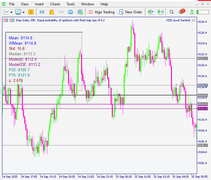
Figure below shows the EA’s statistical panel and corresponding horizontal levels plotted on the Step Index (M5). The mean and weighted mean converge at 8114.8, establishing a stable central balance point. The standard deviation (15.6) indicates moderate volatility within the current sample, while the median (8113.3) remains close to the mean, reflecting a symmetric distribution of prices. Both the discrete mode (8112.4) and the KDE-estimated mode (8113.2) cluster just below the mean, marking a dense trading zone that functions as a natural support/resistance region. The percentiles (P25 = 8105.7, P75 = 8121.6) capture the interquartile range of 16 points, effectively framing the middle 50% of activity and highlighting the consolidation band where price oscillates most frequently. Finally, the z-score (2.676) shows that price has moved more than two standard deviations above the mean, suggesting temporary overextension and increasing the likelihood of mean reversion.

Together, these results demonstrate how statistical levels derived from Typical Price can serve as actionable reference points. The EA’s on-chart display allows traders to visually confirm whether market behavior respects, rejects, or overshoots these zones, making it easier to align trading decisions with objectively measured structure rather than subjective judgment.

Conclusion

The EA computes distributional reference levels from Typical Price (TP = (H+L+C)/3) and publishes them directly on the chart: labeled horizontal lines (mean, weighted mean, median, binned & KDE modes, P25/P75), a compact metrics panel, and visual signals (arrows, touch/outcome markers). It also exports globals for programmatic use and includes monitoring logic that records touches and classifies outcomes as breakout, reversal or no-follow.

These levels convert clustering, central tendency and dispersion into objective, on-chart reference points you can read at a glance, think of them as a statistical map of recent price behavior. Use them as decision-support: confirm how price interacts with these zones before acting, and treat the EA’s outputs as context, not automatic trade execution. In future projects we will explore more advanced statistical methods and ensemble techniques to improve level stability and predictive power.

See my other articles.