Neural Networks in Trading: A Hybrid Trading Framework with Predictive Coding (StockFormer)

Introduction

Reinforcement Learning (RL) is increasingly being applied to complex problems in finance, including the development of trading strategies and portfolio management. Models are trained to analyze historical data on asset price movements, trading volumes, and technical indicators. However, most existing methods assume that the analyzed data fully capture all interdependencies between assets. In practice, this is rarely the case, especially in noisy and highly volatile market environments.

Traditional approaches often fail to account for both short- and long-term return forecasts as well as correlations across assets. Yet, successful investment strategies typically rely on a deep understanding of these factors. To address this, the paper "StockFormer: Learning Hybrid Trading Machines with Predictive Coding" introduces StockFormer, a hybrid trading system that combines predictive coding with the flexibility of RL agents. Predictive coding that is widely used in natural language processing and computer vision, enables the extraction of informative hidden states from noisy input data, a capability that is particularly valuable in financial applications.

The StockFormer integrates three modified Transformer branches, each responsible for capturing different aspects of market dynamics:

• Long-term trends
• Short-term trends
• Cross-asset dependencies

Each branch incorporates a Diversified Multi-Head Attention (DMH-Attn) mechanism, which extends the vanilla Transformer by replacing a single FeedForward block with multiple parallel blocks. This enables the model to capture diverse temporal patterns across subspaces while preserving critical information.

To optimize trading strategies, the latent states produced by these three branches are adaptively fused using multi-head attention into a unified state space, which is then used by the RL agent.

Policy learning is carried out using the Actor–Critic method. Crucially, gradient feedback from the Critic is propagated back to improve the predictive coding module, ensuring tight integration between predictive modeling and policy optimization.

Experiments conducted on three public datasets demonstrated that StockFormer significantly outperforms existing methods in both predictive accuracy and investment returns.

The StockFormer algorithm

StockFormer addresses forecasting and trading decision-making in financial markets through RL. A key limitation of conventional methods lies in their inability to effectively model dynamic dependencies between assets and their future trends. This is especially important in markets where conditions change rapidly and unpredictably. StockFormer resolves this challenge through two core stages: predictive coding and trading strategy learning.

In the first stage, StockFormer leverages self-supervised learning to extract hidden patterns from noisy market data. This allows the model to capture short- and long-term dynamics as well as cross-asset dependencies. Using this approach, the model extracts important hidden states, which are then used in the next step to make trading decisions.

Financial markets exhibit highly diverse temporal patterns across multiple assets, complicating the extraction of effective representations from raw data. To address this, StockFormer modifies the vanilla Transformer's multi-head attention mechanism by replacing the single FeedForward network (FFN) with a group of parallel FFNs. Without increasing the parameter count, this design strengthens the ability of multi-head attention to decompose features, thereby improving the modeling of heterogeneous temporal patterns across subspaces.

This enhanced module is called Diversified Multi-Head Attention (DMH-Attn). For Query, Key, and Value entities of dimension dmodel, the process begins by splitting the output features Z of multi-head attention into h groups along the channel dimension, where h is the number of attention heads. A dedicated FFN is then applied to each group in Z:

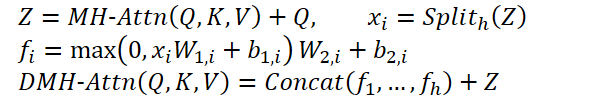
Here MH-Attn indicates multi-head attention. 𝑓𝑖 are output features of each FFN head, containing two linear projections with ReLU activation between them.

Each branch in the modernized Transformer in StockFormer is divided into two modules: an encoder and a decoder. Both are used during predictive coding training, but only the encoder is employed during strategy optimization. The model comprises L encoder layers and M decoder layers. The final encoder output XLenc is fed into each decoder layer. The process of calculations on the l-th encoder layer and m-th decoder layer can be written as follows:

• encoder layer:

• decoder layer:

Here Xl,enc and Xm,dec are encoder and decoder outputs, respectively. Inputs to the first encoder and decoder layers consist of raw data with positional embeddings. The final decoder output is passed through a projection layer to generate predictive coding results.

The cross-asset dependency module identifies dynamic correlations across time series. At each time step t, it processes identical inputs in both encoder and decoder. For stock market data, the framework authors used technical indicators such as MACD, RSI, and SMA.

During training, data are split into two parts:

1. Covariance matrix. The covariance matrix is computed across daily closing prices of all assets over a fixed window before time t.
2. Masked statistics. This part contains half of the time series are randomly masked with zeros, while the remainder serve as visible features. At test time, we use full (unmasked) data.

The goal is to reconstruct masked statistics based on the covariance matrix and the remaining features. This predictive coding task forces the Transformer encoder to learn interdependencies across assets.

Short-term and long-term forecasting modules in StockFormer aim at predicting the return rates for each asset over different time horizons.

The short-term forecasting module predicts next-day returns for the asset (H = 1). For this, we feed analyzed statistics for T days into the encoder. The decoder receives the same statistics but for the analyzed moment in time.

The long-term module operates similarly but returns forecasts over a longer horizon. This encourages the model to capture extended market dynamics.

For training the short-term and long-term forecasting modules, a combined loss function is used, incorporating both regression error and stock ranking error. The regression error minimizes the gap between predicted and actual returns, while the ranking error ensures that assets with higher returns are prioritized.

Thus, the two branches of the model enable StockFormer to capture market dynamics across different time horizons, allowing the RL agent to make more accurate and better-informed trading decisions.

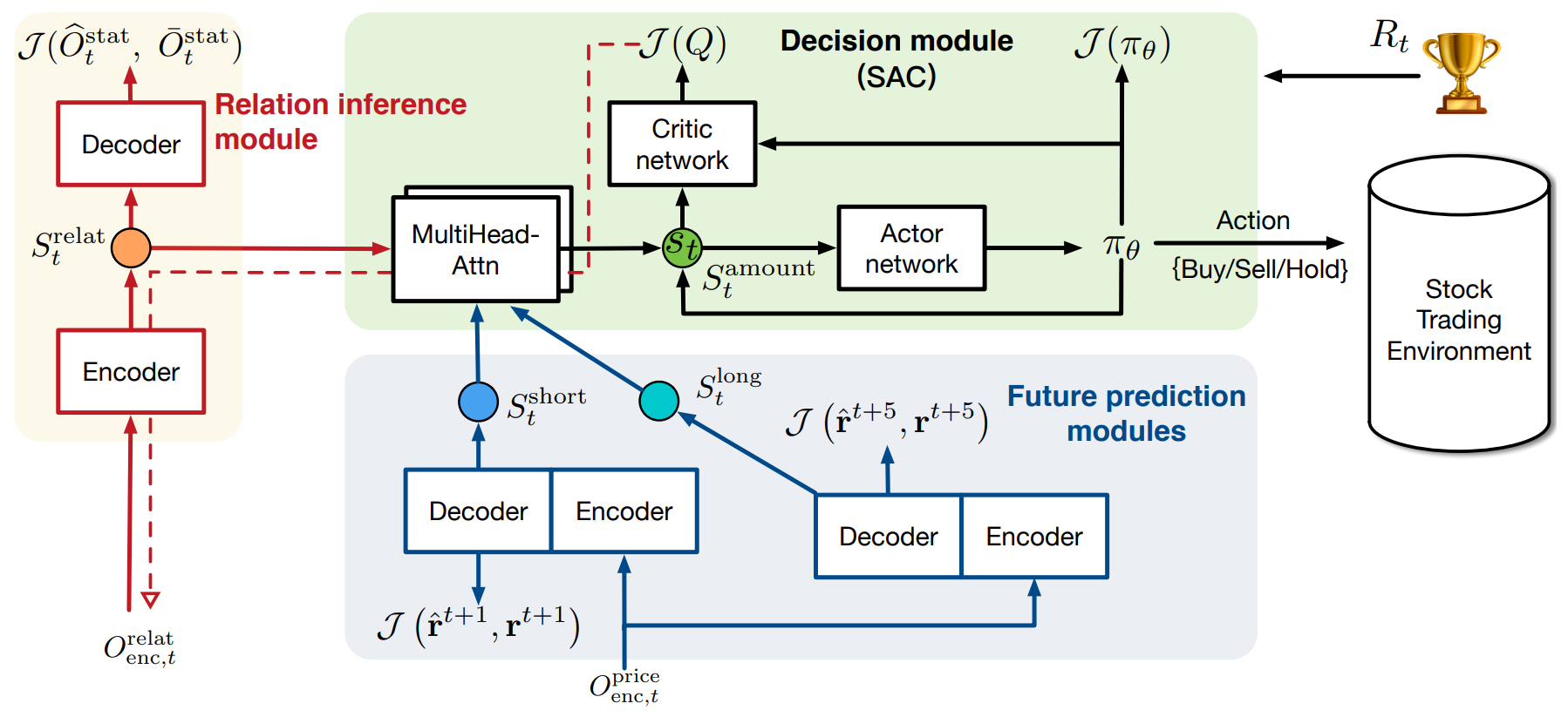
In the second training stage, StockFormer integrates three types of latent representations: srelat,t, slong,t, and sshort,t into a unified state space St using a cascade of multi-head attention blocks. The process begins with the fusion of short-term and long-term forecasts. Here, the long-term forecast representation serves as the Query, as it is less affected by short-term noise. The outcome of this step is then aligned with the latent representation of asset interdependencies, which is used as the Key and Value in the subsequent attention module.

The model is then trained to determine the optimal trading strategy using the Actor–Critic approach. One of the key advantages of StockFormer is the integration of predictive coding and policy optimization phases. The Critic's evaluations help refine the quality of latent representation extraction, enabling the model to analyze inter-asset relationships more effectively and to better handle noise in the input data.

The original visualization of the StockFormer framework is provided below.

Implementation in MQL5

After covering the theoretical foundation of StockFormer, we turn to implementing the proposed methods in MQL5. As highlighted in the theoretical description, the key architectural modification lies in introducing a multi-head FeedForward block. Implementing this block is the first step of our work.

In the implementation of the multi-head FeedForward block proposed by the authors of the StockFormer framework, the outputs of the multi-head Self-Attention block for each sequence element are divided into h equal groups, with each group processed by its own MLP with unique trainable parameters.

It is important to note that the approach to forming heads here differs from the one used in the conventional multi-head attention block. In Multi-Head Self-Attention, multiple versions of Query, Key, and Value entities were generated from a single sequence element embedding. In this case, however, the authors of StockFormer propose splitting the representation vector of a sequence element directly into several equal groups. Each group is then processed by its own MLP. This approach, of course, enables the creation of multiple heads without increasing the number of trainable parameters. Moreover, the output tensor preserves the same dimensionality, eliminating the need for a projection layer as in MH Self-Attention. However, because of this, we cannot use existing convolutional layers, as was possible before. This means we must find an alternative solution.

On the one hand, we could consider transposing the three-dimensional tensor to adapt the solution for convolutional layers with independent analysis of unidimensional sequences. But StockFormer contains a substantial number of such layers. Therefore, transposing data before and after the FeedForward block at each layer would significantly increase both training and inference time. Therefore, the decision was made to design a multi-head variant of the convolutional layer. Before implementing this new component in the main program, however, some adjustments are required on the OpenCL side.

Extending the OpenCL Program

We begin by constructing the feed-forward-pass kernel for the new multi-head convolutional FeedForwardMHConv layer. It should be noted that the parameter structure and part of the algorithm were borrowed from the kernel of the existing convolutional layer. The convolutional head identifier and the total number of heads were introduced as an additional dimension in the task space.

__kernel void FeedForwardMHConv(__global float *matrix_w,
                                __global float *matrix_i,
                                __global float *matrix_o,
                                const int inputs,
                                const int step,
                                const int window_in,
                                const int window_out,
                                const int activation
                               )
  {
   const size_t i = get_global_id(0);
   const size_t h = get_global_id(1);
   const size_t v = get_global_id(2);
   const size_t total = get_global_size(0);
   const size_t heads = get_global_size(1);

In the kernel body we identify the thread across all dimensions of the task space. We then determine the input and output dimensions for each convolution head, as well as the offsets in the global data buffers corresponding to the elements under analysis.

   const int window_in_h = (window_in + heads - 1) / heads;
   const int window_out_h = (window_out + heads - 1) / heads;
   const int shift_out = window_out * i + window_out_h * h;
   const int shift_in = step * i + window_in_h * h;
   const int shift_var_in = v * inputs;
   const int shift_var_out = v * window_out * total;
   const int shift_var_w = v * window_out * (window_in_h + 1);
   const int shift_w_h = h * window_out_h * (window_in_h + 1);

Once this preparatory work is complete, we move on to constructing the convolution operations between the input data and the trainable filter. Within a single thread, we perform convolution for one head of the input data with its corresponding filter. To achieve this, we organize a system of nested loops. The outer loop iterates over the elements of the output layer corresponding to the given convolution head.

   float sum = 0;
   float4 inp, weight;
   int stop = (window_in_h <= (inputs - shift_in) ? window_in_h : (inputs - shift_in));
//---
   for(int out = 0; (out < window_out_h && (window_out_h * h + out) < window_out); out++)
     {
      int shift = (window_in_h + 1) * out + shift_w_h;

Within the outer loop, we first calculate the offset in the buffer of trainable parameters. We then initiate an inner loop to traverse the elements of the convolution window applied to the input data.

      for(int k = 0; k <= stop; k += 4)
        {
         switch(stop - k)
           {
            case 0:
               inp = (float4)(1, 0, 0, 0);
               weight = (float4)(matrix_w[shift_var_w + shift + window_in_h], 0, 0, 0);
               break;
            case 1:
               inp = (float4)(matrix_i[shift_var_in + shift_in + k], 1, 0, 0);
               weight = (float4)(matrix_w[shift_var_w + shift + k], matrix_w[shift_var_w + shift + window_in_h], 0, 0);
               break;
            case 2:
               inp = (float4)(matrix_i[shift_var_in + shift_in + k],
                              matrix_i[shift_var_in + shift_in + k + 1], 1, 0);
               weight = (float4)(matrix_w[shift_var_w + shift + k], matrix_w[shift_var_w + shift + k + 1],
                                 matrix_w[shift_var_w + shift + window_in_h], 0);
               break;
            case 3:
               inp = (float4)(matrix_i[shift_var_in + shift_in + k], matrix_i[shift_var_in + shift_in + k + 1],
                              matrix_i[shift_var_in + shift_in + k + 2], 1);
               weight = (float4)(matrix_w[shift_var_w + shift + k], matrix_w[shift_var_w + shift + k + 1],
                                 matrix_w[shift_var_w + shift + k + 2], matrix_w[shift_var_w + shift + shift_w_h]);
               break;
            default:
               inp = (float4)(matrix_i[shift_var_in + shift_in + k], matrix_i[shift_var_in + shift_in + k + 1],
                              matrix_i[shift_var_in + shift_in + k + 2], matrix_i[shift_var_in + shift_in + k + 3]);
               weight = (float4)(matrix_w[shift_var_w + shift + k], matrix_w[shift_var_w + shift + k + 1],
                                 matrix_w[shift_var_w + shift + k + 2], matrix_w[shift_var_w + shift + k + 3]);
               break;
           }

To optimize computation, we use built-in vector multiplication functions, which allow for more efficient use of processor resources. Accordingly, we first load the necessary values from external buffers into local vector variables, then perform vector multiplications before moving on to the next iteration of the inner loop.

         sum += IsNaNOrInf(dot(inp, weight), 0);
        }

After completing all iterations of the inner loop, we apply the activation function and store the result in the corresponding output buffer element. The process then continues with the next iteration of the outer loop.

      sum = IsNaNOrInf(sum, 0);
      //---
      matrix_o[shift_var_out + out + shift_out] = Activation(sum, activation);;
     }
  }

By the end of all loop iterations, the output buffer contains all required values, and the kernel execution is complete.

We now proceed to constructing the backpropagation algorithms. Here, it must be noted that unlike in the feed-forward pass, we cannot introduce the convolution head identifier as a dimension in the task space.

Recall that during the gradient distribution process, we accumulate the influence values of each input element on the output. In cases where the stride of the convolution window is smaller than its size, a single input element may affect result tensor elements across multiple convolution heads.

For this reason, in this case, we introduce the number of attention heads as an additional external parameter of the CalcHiddenGradientMHConv kernel. The identifier of the specific convolution head is then determined during the process of accumulating the error gradients.

__kernel void CalcHiddenGradientMHConv(__global float *matrix_w,
                                       __global float *matrix_g,
                                       __global float *matrix_o,
                                       __global float *matrix_ig,
                                       const int outputs,
                                       const int step,
                                       const int window_in,
                                       const int window_out,
                                       const int activation,
                                       const int shift_out,
                                       const int heads
                                      )
  {
   const size_t i = get_global_id(0);
   const size_t inputs = get_global_size(0);
   const size_t v = get_global_id(1);

In the kernel body, we identify the current thread in the two-dimensional task space, which points to the input data element and the univariate sequence identifier. After that, we determine the values of the constants, including shift in the data buffers, as well as the window dimensions and the number of filters for one convolution head. 

   const int shift_var_in = v * inputs;
   const int shift_var_out = v * outputs;
   const int shift_var_w = v * window_out * (window_in + 1);
   const int window_in_h = (window_in + heads - 1) / heads;
   const int window_out_h = (window_out + heads - 1) / heads;

Here we also define the range of the output window that is influenced by the analyzed element of the source data.

   float sum = 0;
   float out = matrix_o[shift_var_in + i];
   const int w_start = i % step;
   const int start = max((int)((i - window_in + step) / step), 0);
   int stop = (w_start + step - 1) / step;
   stop = min((int)((i + step - 1) / step + 1), stop) + start;
   if(stop > (outputs / window_out))
      stop = outputs / window_out;

After the preparatory work, we proceed to collecting error gradients from all dependent elements of the result tensor. To achieve this, we organize a system of loops. The outer loop will iterate over dependent elements within the previously defined window.

   for(int k = start; k < stop; k++)
     {
      int head = (k % window_out) / window_out_h;

In the body of the outer loop, we first define the convolution head for a single element of the result tensor, and then organize a nested loop for iterating over filters.

      for(int h = 0; h < window_out_h; h ++)
        {
         int shift_g = k * window_out + head * window_out_h + h;
         int shift_w = (stop - k - 1) * step + (i % step) / window_in_h +
                       head * (window_in_h + 1) + h * (window_in_h + 1);
         if(shift_g >= outputs || shift_w >= (window_in_h + 1) * window_out)
            break;
         float grad = matrix_g[shift_out + shift_g + shift_var_out];
         sum += grad * matrix_w[shift_w + shift_var_w];
        }
     }

It is within the body of the nested loop that we accumulate the error gradient across all filters of a single convolution head before moving on to the next iteration of the loop system.

Once the gradients from all dependent elements have been collected, the accumulated value is adjusted by the derivative of the activation function and the result is stored in the corresponding element of the data buffer:

   matrix_ig[shift_var_in + i] = Deactivation(sum, out, activation);
  }

At this point, the operations of the gradient distribution kernel are complete. As for the parameter update kernel, I suggest that you review it independently. The complete OpenCL program code is provided in the appendix to this article. We will now move on to the next stage of our work: implementing the multi-head convolutional neural layer in the main program.

Multi-Head Convolutional Layer

To implement the convolutional functionality on the main program side, we introduce a new object, CNeuronMHConvOCL. As one might expect, the existing convolutional layer was used as the parent class. The structure of the new object is presented below.

class CNeuronMHConvOCL  :  public CNeuronConvOCL
  {
protected:
   uint              iHeads;
   //---
   virtual bool      feedForward(CNeuronBaseOCL *NeuronOCL) override;
   virtual bool      updateInputWeights(CNeuronBaseOCL *NeuronOCL) override;
   virtual bool      calcInputGradients(CNeuronBaseOCL *NeuronOCL) override;

public:
                     CNeuronMHConvOCL(void)  :  iHeads(1)   {};
                    ~CNeuronMHConvOCL(void)  {};
   //---
   virtual bool      Init(uint numOutputs, uint myIndex, COpenCLMy *open_cl, 
                          uint window, uint step, uint window_out, 
                          uint units_count, uint variables, uint heads, 
                          ENUM_OPTIMIZATION optimization_type, uint batch);
   //---
   virtual int       Type(void)   const override   {  return defNeuronMHConvOCL;   }
   //--- methods for working with files
   virtual bool      Save(int const file_handle) override;
   virtual bool      Load(int const file_handle) override;
  };

In this structure, only one internal variable is introduced to store the specified number of convolution heads. All other objects and variables required for processing are inherited from the parent class. In addition, the forward and backward pass methods are overridden, serving as wrappers for calling the kernels described earlier. The kernel scheduling algorithm remains unchanged and therefore does not require further explanation. In this article, we will focus exclusively on the initialization method Init, which was implemented almost entirely from scratch.

Within the method's parameter structure, only a single new element was added, enabling the number of convolution heads to be passed from the calling program.

bool CNeuronMHConvOCL::Init(uint numOutputs, uint myIndex, COpenCLMy *open_cl, 
                            uint window, uint step, uint window_out, 
                            uint units_count, uint variables, uint heads, 
                            ENUM_OPTIMIZATION optimization_type, uint batch)
  {
   if(!CNeuronProofOCL::Init(numOutputs, myIndex, open_cl, window, step, 
                             units_count * window_out * variables, ADAM, batch))
      return false;

Inside the method, we first invoke the corresponding initialization method of the parent subsampling layer, which in this case acts as the ancestral object. We then assign the values of the external parameters to local variables.

   iWindowOut = window_out;
   iVariables = variables;
   iHeads = MathMax(MathMin(heads, window), 1);

Next, we must initialize the tensor of trainable parameters with random values. Before doing so, however, we define the dimensionality of this tensor. Its size depends on the number of univariate series in the multimodal sequence under analysis, the total number of filters, and the size of the convolution window for a single head.

   const int window_h = int((iWindow + heads - 1) / heads);
   const int count = int((window_h + 1) * iWindowOut * iVariables);

Note that we are referring to the total number of filters across all convolution heads while using only the convolution window of a single head. It is straightforward to deduce that the number of trainable parameters for a single convolution head equals the product of the number of filters per head and the size of its input window, plus one bias term (Fi * (Wi + 1)). To obtain the total number of parameters for a single univariate sequence, we simply multiply this value by the number of heads (Fi * (Wi + 1) * H). It is also evident that the number of filters per head, multiplied by the number of heads, yields the total number of filters specified by the user.

The next step is to check the validity of the pointer to the buffer object containing the trainable parameters and, if necessary, create a new object.

   if(!WeightsConv)
     {
      WeightsConv = new CBufferFloat();
      if(!WeightsConv)
         return false;
     }

We reserve the required number of elements in the buffer and organize a loop to populate the buffer with random values.

   if(!WeightsConv.Reserve(count))
      return false;
   float k = (float)(1 / sqrt(window_h + 1));
   for(int i = 0; i < count; i++)
     {
      if(!WeightsConv.Add((GenerateWeight() * 2 * k - k) * WeightsMultiplier))
         return false;
     }
   if(!WeightsConv.BufferCreate(OpenCL))
      return false;

After successfully filling the buffer with random values, we transfer it to the OpenCL context memory. Next, we create momentum buffers, filling them with zero values.

   if(!FirstMomentumConv)
     {
      FirstMomentumConv = new CBufferFloat();
      if(!FirstMomentumConv)
         return false;
     }
   if(!FirstMomentumConv.BufferInit(count, 0.0))
      return false;
   if(!FirstMomentumConv.BufferCreate(OpenCL))
      return false;
//---
   if(!SecondMomentumConv)
     {
      SecondMomentumConv = new CBufferFloat();
      if(!SecondMomentumConv)
         return false;
     }
   if(!SecondMomentumConv.BufferInit(count, 0.0))
      return false;
   if(!SecondMomentumConv.BufferCreate(OpenCL))
      return false;
   if(!!DeltaWeightsConv)
      delete DeltaWeightsConv;
//---
   return true;
  }

At this point, we conclude our discussion of the methods of the multi-head convolutional layer object CNeuronMHConvOCL. The full implementation of this class and all of its methods can be found in the appendix.

Multi-Head FeedForward Block

We have now created the first building block in the construction of the StockFormer framework. Next, we will use it to implement the multi-head FeedForward block within the new object CNeuronMHFeedForward, whose structure is shown below.

class CNeuronMHFeedForward   :  public CNeuronBaseOCL
  {
protected:
   CNeuronMHConvOCL  acConvolutions[2];
   //---
   virtual bool      feedForward(CNeuronBaseOCL *NeuronOCL) override;
   virtual bool      updateInputWeights(CNeuronBaseOCL *NeuronOCL) override;
   virtual bool      calcInputGradients(CNeuronBaseOCL *NeuronOCL) override;

public:
                     CNeuronMHFeedForward(void) {};
                    ~CNeuronMHFeedForward(void) {};
   //---
   virtual bool      Init(uint numOutputs, uint myIndex, COpenCLMy *open_cl,
                          uint window, uint window_out,
                          uint units_count, uint variables, uint heads,
                          ENUM_OPTIMIZATION optimization_type, uint batch);
   //---
   virtual int       Type(void)   const override   {  return defNeuronMHFeedForward;   }
   //--- methods for working with files
   virtual bool      Save(int const file_handle) override;
   virtual bool      Load(int const file_handle) override;
   //---
   virtual void      SetOpenCL(COpenCLMy *obj) override;
  };

In the structure of the new object, we declare an array consisting of two internal multi-head convolutional layers and override the familiar set of virtual methods. These internal objects are declared statically, which allows us to keep the constructor and destructor empty. Initialization of all declared and inherited objects is performed in the Init method.

bool CNeuronMHFeedForward::Init(uint numOutputs, uint myIndex, COpenCLMy *open_cl,
                                uint window, uint window_out,
                                uint units_count, uint variables, uint heads,
                                ENUM_OPTIMIZATION optimization_type, uint batch)
  {
   if(!CNeuronBaseOCL::Init(numOutputs, myIndex, open_cl, window * units_count * variables, optimization_type, batch))
      return false;

The initialization method receives constants that define the architecture of the object being created. Some of these parameters are immediately passed to the corresponding initialization method of the parent class to set up the inherited base interfaces.

We then initialize the first convolutional layer, specifying GELU as its activation function.

   if(!acConvolutions[0].Init(0, 0, OpenCL, window, window, window_out, units_count, variables, heads, 
                                                                                  optimization, iBatch))
      return false;
   acConvolutions[0].SetActivationFunction(GELU);

After that, we initialize the second convolutional layer, this time without an activation function.

   if(!acConvolutions[1].Init(0, 1, OpenCL, window_out, window_out, window, units_count, variables, heads, 
                                                                                     optimization, iBatch))
      return false;
   acConvolutions[1].SetActivationFunction(None);

It should be noted that when calling the initialization method of the second convolutional layer, we swap the parameters corresponding to the number of filters and the input window size.

At the output of the FeedForward block, residual connections with normalization are applied. For this reason, we do not override the result buffer of the block's interface. However, we do override the error gradient buffer, enabling direct transfer of gradients from the interfaces into the corresponding buffer of the second convolutional layer.

   if(!SetGradient(acConvolutions[1].getGradient(), true))
      return false;
   SetActivationFunction(None);
//---
   return true;
  }

We also disable the activation function for the block itself and complete the initialization method by returning the logical result of execution to the calling program.

Once initialization is complete, we move on to implementing the forward-pass algorithm within the feedForward method. In this case, the implementation is straightforward. We simply invoke the forward-pass methods of the internal convolutional layers in sequence.

bool CNeuronMHFeedForward::feedForward(CNeuronBaseOCL *NeuronOCL)
  {
   CObject *prev = NeuronOCL;
   for(uint i = 0; i < acConvolutions.Size(); i++)
     {
      if(!acConvolutions[i].FeedForward(prev))
         return false;
      prev = GetPointer(acConvolutions[i]);
     }

The outputs are then summed with the original inputs, followed by normalization within the elements of the multimodal sequence under analysis.

   if(!SumAndNormilize(NeuronOCL.getOutput(), acConvolutions[acConvolutions.Size() - 1].getOutput(),
                       Output, acConvolutions[0].GetWindow(), true, 0, 0, 0, 1))
      return false;
//---
   return true;
  }

The method concludes by returning the logical result of the operation to the calling program.

The calcInputGradients algorithm of the error gradient distribution method looks a little more complicated since we need to propagate gradients along two data streams.

bool CNeuronMHFeedForward::calcInputGradients(CNeuronBaseOCL *NeuronOCL)
  {
   if(!NeuronOCL)
      return false;

The parameters of this method include a pointer to the source data object; into its buffer we WILL pass the error gradient, distributed in accordance with the influence of the input data on the final model output. And in the method body, we immediately check the relevance of the received pointer.

After successfully passing the control block, we organize a loop of the reverse iteration through the internal convolutional layers while sequentially calling the relevant methods.

   for(int i = (int)acConvolutions.Size() - 2; i >= 0; i--)
     {
      if(!acConvolutions[i].calcHiddenGradients(acConvolutions[i + 1].AsObject()))
         return false;
     }

After the error gradient is distributed across the internal object pipeline, it is then propagated to the source data level. This operation concludes the main workflow.

   if(!NeuronOCL.calcHiddenGradients(acConvolutions[0].AsObject()))
      return false;

Next, we need to propagate the error gradient along the second information stream. The algorithm here is split into two branches of operations, depending on the presence of the activation function of the source data. Since we don't have an activation function, we simply sum the accumulated error gradient at the source data level with similar values at the output of our block.

   if(NeuronOCL.Activation() == None)
     {
      if(!SumAndNormilize(NeuronOCL.getGradient(), Gradient, NeuronOCL.getGradient(),
                          acConvolutions[0].GetWindow(), false, 0, 0, 0, 1))
         return false;
     }
   else
     {
      if(!DeActivation(NeuronOCL.getOutput(), NeuronOCL.getPrevOutput(), Gradient, NeuronOCL.Activation()) ||
         !SumAndNormilize(NeuronOCL.getGradient(), NeuronOCL.getPrevOutput(), NeuronOCL.getGradient(),
                          acConvolutions[0].GetWindow(), false, 0, 0, 0, 1))
         return false;
     }
//---
   return true;
  }

Otherwise, we would need to first adjust the error gradient of our block's output level by the derivative of the activation function of the source data. Only then would we sum the data from the two information streams.

All that remains is to return the result of the operations to the calling program and exit the method.

The method for adjusting the trainable parameters of the block toward reducing the overall model error, updateInputWeights, is left for independent study. Its algorithm is quite straightforward: we simply call the corresponding methods of the internal objects in sequence. The complete implementation of the multi-head FeedForward block object CNeuronMHFeedForward, along with all its methods, can be found in the attachment to this article.

Decoder of Diversified Multi-Head Attention

After building the multi-head FeedForward block, we now proceed to the construction of encoder and decoder objects for diversified multi-head attention. To implement the algorithms of these modules, we introduce new objects: CNeuronDMHAttention and CNeuronCrossDMHAttention, respectively. The construction of these objects follows a largely similar structure. The latter, however, differs in that it contains an internal cross-attention block and operates with two sources of input data. Within the scope of this article, I propose focusing on the decoder as the more complex object. Once its algorithms are clear, understanding the encoder will not pose significant difficulty.

As the parent class for both objects, we use CNeuronRMAT, which provides the underlying algorithm of the sequential model.

class CNeuronCrossDMHAttention   :  public CNeuronRMAT
  {
protected:
   //---
   virtual bool      feedForward(CNeuronBaseOCL *NeuronOCL) override { return false; }
   virtual bool      feedForward(CNeuronBaseOCL *NeuronOCL, CBufferFloat *SecondInput) override;
   virtual bool      calcInputGradients(CNeuronBaseOCL *prevLayer) override { return false; }
   virtual bool      calcInputGradients(CNeuronBaseOCL *NeuronOCL, CBufferFloat *SecondInput,
                                                                   CBufferFloat *SecondGradient, 
                                                        ENUM_ACTIVATION SecondActivation = None) override;
   virtual bool      updateInputWeights(CNeuronBaseOCL *NeuronOCL) override { return false; }
   virtual bool      updateInputWeights(CNeuronBaseOCL *NeuronOCL, CBufferFloat *SecondInput) override;

public:
                     CNeuronCrossDMHAttention(void)  {};
                    ~CNeuronCrossDMHAttention(void)  {};
   //---
   virtual bool      Init(uint numOutputs, uint myIndex, COpenCLMy *open_cl,
                          uint window, uint window_key, uint units_count,
                          uint window_cross, uint units_cross,
                          uint heads, uint layers,
                          ENUM_OPTIMIZATION optimization_type, uint batch);
   //---
   virtual int       Type(void) override   const   {  return defNeuronCrossDMHAttention; }
  };

In the structure of the decoder object, we can observe only the overriding of virtual methods. The internal object structure is defined in the initialization method Init, whose parameters include the key constants that determine the architecture of the object.

bool CNeuronCrossDMHAttention::Init(uint numOutputs, uint myIndex, COpenCLMy *open_cl,
                                    uint window, uint window_key, uint units_count,
                                    uint window_cross, uint units_cross, uint heads,
                                    uint layers, ENUM_OPTIMIZATION optimization_type, uint batch)
  {
   if(!CNeuronBaseOCL::Init(numOutputs, myIndex, open_cl, window * units_count, optimization_type, batch))
      return false;

In the body of the method, we first invoke the parent class’s initialization method of the fully connected layer to set up the inherited interfaces.

Next, we clear the dynamic array used for storing pointers to the internal objects of the module and create several local variables for temporary data storage.

   cLayers.Clear();
   cLayers.SetOpenCL(OpenCL);
   CNeuronRelativeSelfAttention *attention = NULL;
   CNeuronRelativeCrossAttention *cross = NULL;
   CNeuronMHFeedForward *conv = NULL;
   bool use_self = units_count > 0;
   int layer = 0;

Once this preparatory stage is complete, we organize a loop with the number of iterations equal to the specified number of internal layers of the diversified multi-head attention decoder.

   for(uint i = 0; i < layers; i++)
     {
      if(use_self)
        {
         attention = new CNeuronRelativeSelfAttention();
         if(!attention ||
            !attention.Init(0, layer, OpenCL, window, window_key, units_count, heads, optimization, iBatch) ||
            !cLayers.Add(attention)
           )
           {
            delete attention;
            return false;
           }
         layer++;
        }

Inside the loop, we first create a block of relative Self-Attention to analyze dependencies in the primary input data stream. It is important to note that the Self_Attention block is instantiated only when the sequence length of the primary input stream is greater than "1". Otherwise, there is no data available for dependency analysis.

We then add a relative cross-attention module.

      cross = new CNeuronRelativeCrossAttention();
      if(!cross ||
         !cross.Init(0, layer, OpenCL, window, window_key, units_count, heads, 
                              window_cross, units_cross, optimization, iBatch) ||
         !cLayers.Add(cross)
        )
        {
         delete cross;
         return false;
        }
      layer++;

Each internal layer of the decoder is completed with a multi-head FeedForward block, after which we move on to the next iteration of the loop.

      conv = new CNeuronMHFeedForward();
      if(!conv ||
         !conv.Init(0, layer, OpenCL, window, 2 * window, units_count, 1, heads, optimization, iBatch) ||
         !cLayers.Add(conv)
        )
        {
         delete conv;
         return false;
        }
      layer++;
     }

After initializing the full set of internal objects, we replace the interface pointers with references to these objects and conclude the method, returning a logical result to the calling program.

   SetOutput(conv.getOutput(), true);
   SetGradient(conv.getGradient(), true);
//---
   return true;
  }

The algorithm of the feedForward method consists of sequential calls to the respective methods of the internal objects. I suggest leaving its study as an independent exercise. Instead, let's dedicate some attention to the error gradient distribution algorithm calcInputGradients.

bool CNeuronCrossDMHAttention::calcInputGradients(CNeuronBaseOCL *NeuronOCL, CBufferFloat *SecondInput, 
                                   CBufferFloat *SecondGradient, ENUM_ACTIVATION SecondActivation = -1)
  {
   if(!NeuronOCL || !SecondInput || !SecondGradient)
      return false;

The parameters of this method include pointers to the input data objects and their corresponding error gradients, into which the results of the operations will be written. Therefore, within the method body, we first validate the pointers received.

It is important to highlight that during the feed-forward pass, the second input data source is equally utilized by the cross-attention modules of all decoder layers. Consequently, we must aggregate the error gradients from all information flows. As usual in such cases, we need an internal buffer for data storage. Since no such buffer was defined in the new object, we use one of the unused buffers inherited from the parent class.

First, we check the size of the inherited buffer and, if necessary, adjust it.

   if(PrevOutput.Total() != SecondGradient.Total())
     {
      PrevOutput.BufferFree();
      if(!PrevOutput.BufferInit(SecondGradient.Total(), 0) ||
         !PrevOutput.BufferCreate(OpenCL))
         return false;
     }

Next, we initialize the error gradient buffer for the second data source with zero values. This step ensures that gradients from the current pass are not accumulated with values from previous ones.

   if(!SecondGradient.Fill(0))
      return false;

We then create local variables for temporary data storage.

   CObject *next = cLayers[-1];
   CNeuronBaseOCL *current = NULL;

At this point, the preparatory stage is complete, and we initiate a reverse iteration loop over the internal objects.

   for(int i = cLayers.Total() - 2; i >= 0; i--)
     {
      current = cLayers[i];
      if(!current ||
         !current.calcHiddenGradients(next, SecondInput, PrevOutput, SecondActivation))
         return false;
      if(next.Type() == defNeuronCrossDMHAttention)
         if(!SumAndNormilize(SecondGradient, PrevOutput, SecondGradient, 1, false, 0, 0, 0, 1))
            return false;
      next = current;
     }

Within this loop, we sequentially call the respective methods of the internal objects, while continuously checking the type of the object responsible for distributing the error gradients. If a cross-attention block is encountered, we add the error gradient of the second data source to the previously accumulated values.

After successfully completing all iterations of the loop, we propagate the error gradient back to the input data of the main stream.

   if(!NeuronOCL.calcHiddenGradients(next, SecondInput, PrevOutput, SecondActivation))
      return false;
   if(next.Type() == defNeuronCrossDMHAttention)
      if(!SumAndNormilize(SecondGradient, PrevOutput, SecondGradient, 1, false, 0, 0, 0, 1))
         return false;
//---
   return true;
  }

At this stage, we again verify the type of the object performing the gradient distribution and, if necessary, add the error gradient from the second information stream to the accumulated values. Finally, we conclude the method by returning a logical result to the calling program.

This completes our review of the construction algorithms for the decoder of diversified multi-head attention. The complete implementation of this object and all its methods can be found in the attachment. There you will also find the full code for all other objects presented in this article.

We have now implemented the core architectural unit of the StockFormer framework - the diversified multi-head attention module in the form of both the encoder and decoder of the Transformer architecture. However, the authors of StockFormer also propose a two-level training process with a sophisticated mechanism of interaction between trainable models. This will be discussed in the upcoming article.

Conclusion

We have become familiar with the StockFormer framework, whose authors propose an innovative approach to training trading strategies in financial markets. StockFormer combines methods of predictive coding with deep reinforcement learning. Its primary advantage lies in its ability to train flexible policies that account for dynamic dependencies between multiple assets, while simultaneously predicting their behavior in both short-term and long-term horizons. 

The three-branch predictive coding mechanism extracts latent representations tied to short-term trends, long-term dynamics, and inter-asset dependencies. The cascading multi-head attention mechanism allows for efficient integration of these diverse representations into a unified state space.

In the practical section of this article, we implemented in MQL5 the modification of the vanilla Transformer algorithm proposed by the authors and incorporated it into the encoder and decoder modules of diversified multi-head attention. In the next article, we will continue this work by discussing the architecture of the trainable models and the process of their training.

References

• StockFormer: Learning Hybrid Trading Machines with Predictive Coding
• Other articles from this series

Programs used in the article

#	Name	Type	Description
1	Research.mq5	Expert Advisor	Expert Advisor for collecting samples
2	ResearchRealORL.mq5	Expert Advisor	Expert Advisor for collecting samples using the Real-ORL method
3	Study1.mq5	Expert Advisor	Predictive Learning Expert Advisor
4	Study2.mq5	Expert Advisor	Policy Training Expert Advisor
5	Test.mq5	Expert Advisor	Model testing Expert Advisor
6	Trajectory.mqh	Class library	System state description structure
7	NeuroNet.mqh	Class library	A library of classes for creating a neural network
8	NeuroNet.cl	Code Base	OpenCL program code library