Quantum computing and trading: A fresh approach to price forecasts

Introduction to quantum computing for trading: Key concepts and benefits

Imagine a world where every market transaction is analyzed through the lens of possibilities that exist simultaneously — like famous Schrödinger's cat who is both alive and dead until we open the box. This is how quantum trading works: it looks at all potential market states at once, opening up new horizons for financial analysis.

While conventional computers handle information sequentially, bit by bit, quantum systems exploit the amazing properties of the microworld – superposition and entanglement – to analyze multiple scenarios in parallel. It is like an experienced trader who keeps dozens of charts, news and indicators in his head at the same time, but scaled up to unimaginable limits.

We live in an era where algorithmic trading has already become the norm, but now we are on the cusp of the next revolution. Quantum computing promises more than just faster data analysis — it offers a fundamentally new approach to understanding market processes. Imagine that instead of predicting the price of an asset linearly, we could explore an entire tree of probability scenarios, where each branch takes into account the most subtle market correlations.

In this article, we will dive into the world of quantum trading - from the basic principles of quantum computing to the practical implementation of trading systems. We will look at how quantum algorithms can find patterns where conventional methods fail, and how this advantage can be applied to making trading decisions in real time.

Our journey will start with the basics of quantum computing and gradually lead us to creating a working market prediction system. Along the way, we will break down complex concepts into simple examples and see how the theoretical benefits of quantum computing translate into practical trading tools.

Quantum superposition and entanglement in the context of financial time series analysis

When analyzing financial markets, we are faced with a fundamental problem: an infinite number of mutually influencing factors. Every price movement is the result of a complex interaction of thousands of variables, from macroeconomic indicators to the sentiment of individual traders. This is where quantum computing offers a unique solution through its fundamental properties – superposition and entanglement.

Let's consider superposition. In a conventional computer, a bit can be either 0 or 1. A qubit exists in all possible states simultaneously until we make a measurement. Mathematically, this is described as |ψ⟩ = α|0⟩ + β|1⟩, where α and β are complex probability amplitudes. When applied to time series analysis, this property allows quantum algorithms to effectively explore the solution space in portfolio and risk management problems by analyzing many potential scenarios in parallel.

Quantum entanglement adds another level of possibility. When qubits are entangled, their states become inextricably linked, as described, for example, by |ψ⟩ = (|00⟩ + |11⟩)/√2. In the context of financial analysis, this property is used in quantum algorithms to model complex correlations between different market indicators. For example, we can create systems that take into account the relationships between asset price, trading volume and market volatility.

These quantum properties are especially useful when working with high-frequency trading, where the speed of handling multidimensional data is critical. Superposition allows for multiple trading scenarios to be analyzed in parallel, while entanglement helps account for complex intermarket correlations in real time. Quantum advantages are most evident in specific optimization and search problems, where classical algorithms face exponential growth in computational complexity.

Developing a quantum forecasting algorithm using QPE (Quantum Phase Estimation)

At the heart of our system lies an elegant combination of quantum computing and classical technical analysis. Imagine a quantum orchestra of eight qubits, where each qubit is a musician playing its part in a complex symphony of market movements.

Everything starts with data preparation. Our quantum predictor receives market data through integration with MetaTrader 5, like neurons collecting information from the senses. This data goes through a normalization process - imagine as if we were tuning all the instruments in an orchestra to the same key.

The most interesting part begins when creating a quantum circuit. First, we put each qubit into a superposition state using Hadamard gates (H-gates). At this point, each qubit exists simultaneously in all possible states, as if each musician were simultaneously playing all possible notes of his part.

We then encode market data into quantum states through ry gates, where the rotation angle is determined by the value of market parameters. It is like a conductor setting the tempo and character of the performance for each musician. Particular attention is paid to the current price - it gets its own quantum twist, influencing the entire system like a soloist in an orchestra.

The real magic happens when quantum entanglement is created. Using cx gates (CNOT), we couple adjacent qubits, creating unbreakable quantum correlations. It is like that moment when the musicians' individual parts merge into a single harmonious sound.

After quantum transformations, we make measurements, as if we were recording a concert. But here is the twist: we repeat this process 2000 times (shots), getting a statistical distribution of the results. Each dimension gives us a bit string, where the number of ones determines the direction of the prediction.

The final chord is the interpretation of the results. The system is very conservative in its forecasts, limiting the maximum price change to 0.1%. It is like an experienced conductor who does not allow the orchestra to play too loud or too soft, maintaining a balance of sound.

The test results speak for themselves. The accuracy of forecasts exceeds random guessing, reaching 54% on the EURUSD H1. At the same time, the system demonstrates a high level of confidence in its forecasts, which is reflected in the 'confidence' metric.

In this implementation, quantum computing does not simply complement classical technical analysis - it creates a new dimension in market analysis, where multiple possible scenarios are explored simultaneously in quantum superposition. As Richard Feynman said: "Nature at the quantum level behaves very differently from what we usually think". And it seems that financial markets also hide a quantum nature that we are only just beginning to understand.

import numpy as np
import MetaTrader5 as mt5
import pandas as pd
from datetime import datetime, timedelta
from qiskit import QuantumCircuit, transpile, QuantumRegister, ClassicalRegister
from qiskit_aer import AerSimulator
from sklearn.preprocessing import MinMaxScaler
from sklearn.metrics import accuracy_score, precision_score, recall_score, f1_score
import warnings
warnings.filterwarnings('ignore')

class MT5DataLoader:
    def __init__(self, symbol="EURUSD", timeframe=mt5.TIMEFRAME_H1):
        if not mt5.initialize():
            raise Exception("MetaTrader5 initialization failed")
        
        self.symbol = symbol
        self.timeframe = timeframe
    
    def get_historical_data(self, lookback_bars=1000):
        current_time = datetime.now()
        rates = mt5.copy_rates_from(self.symbol, self.timeframe, current_time, lookback_bars)
        
        if rates is None:
            raise Exception(f"Failed to get data for {self.symbol}")
            
        df = pd.DataFrame(rates)
        df['time'] = pd.to_datetime(df['time'], unit='s')
        return df

class EnhancedQuantumPredictor:
    def __init__(self, num_qubits=8):  # Reduce the number of qubits for stability
        self.num_qubits = num_qubits
        self.simulator = AerSimulator()
        self.scaler = MinMaxScaler()
        
    def create_qpe_circuit(self, market_data, current_price):
        """Create a simplified quantum circuit"""
        qr = QuantumRegister(self.num_qubits, 'qr')
        cr = ClassicalRegister(self.num_qubits, 'cr')
        qc = QuantumCircuit(qr, cr)
        
        # Normalize data
        scaled_data = self.scaler.fit_transform(market_data.reshape(-1, 1)).flatten()
        
        # Create superposition
        for i in range(self.num_qubits):
            qc.h(qr[i])
        
        # Apply market data as phases
        for i in range(min(len(scaled_data), self.num_qubits)):
            angle = float(scaled_data[i] * np.pi)  # Convert to float
            qc.ry(angle, qr[i])
        
        # Create entanglement
        for i in range(self.num_qubits - 1):
            qc.cx(qr[i], qr[i + 1])
        
        # Apply the current price
        price_angle = float((current_price % 0.01) * 100 * np.pi)  # Use only the last 2 characters
        qc.ry(price_angle, qr[0])
        
        # Measure all qubits
        qc.measure(qr, cr)
        
        return qc
    
    def predict(self, market_data, current_price, features=None, shots=2000):
        """Simplified prediction"""
        # Trim the input data
        if market_data.shape[0] > self.num_qubits:
            market_data = market_data[-self.num_qubits:]
        
        # Create and execute the circuit
        qc = self.create_qpe_circuit(market_data, current_price)
        compiled_circuit = transpile(qc, self.simulator, optimization_level=3)
        job = self.simulator.run(compiled_circuit, shots=shots)
        result = job.result()
        counts = result.get_counts()
        
        # Analyze the results
        predictions = []
        total_shots = sum(counts.values())
        
        for bitstring, count in counts.items():
            # Use the number of ones in the bitstring to determine the direction
            ones = bitstring.count('1')
            direction = ones / self.num_qubits  # Normalized direction
            
            # Predict the change of no more than 0.1%
            price_change = (direction - 0.5) * 0.001
            predicted_price = current_price * (1 + price_change)
            predictions.extend([predicted_price] * count)
        
        predicted_price = np.mean(predictions)
        up_probability = sum(1 for p in predictions if p > current_price) / len(predictions)
        
        confidence = 1 - np.std(predictions) / current_price
        

        
        return {
            'predicted_price': predicted_price,
            'up_probability': up_probability,
            'down_probability': 1 - up_probability,
            'confidence': confidence
        }

class MarketPredictor:
    def __init__(self, symbol="EURUSD", timeframe=mt5.TIMEFRAME_H1, window_size=14):
        self.symbol = symbol
        self.timeframe = timeframe
        self.window_size = window_size
        self.quantum_predictor = EnhancedQuantumPredictor()
        self.data_loader = MT5DataLoader(symbol, timeframe)
    
    def prepare_features(self, df):
        """Prepare technical indicators"""
        df['sma'] = df['close'].rolling(window=self.window_size).mean()
        df['ema'] = df['close'].ewm(span=self.window_size).mean()
        df['std'] = df['close'].rolling(window=self.window_size).std()
        df['upper_band'] = df['sma'] + (df['std'] * 2)
        df['lower_band'] = df['sma'] - (df['std'] * 2)
        df['rsi'] = self.calculate_rsi(df['close'])
        df['momentum'] = df['close'] - df['close'].shift(self.window_size)
        df['rate_of_change'] = (df['close'] / df['close'].shift(1) - 1) * 100
        
        features = df[['sma', 'ema', 'std', 'upper_band', 'lower_band', 
                      'rsi', 'momentum', 'rate_of_change']].dropna()
        return features
    
    def calculate_rsi(self, prices, period=14):
        delta = prices.diff()
        gain = (delta.where(delta > 0, 0)).ewm(alpha=1/period).mean()
        loss = (-delta.where(delta < 0, 0)).ewm(alpha=1/period).mean()
        rs = gain / loss
        return 100 - (100 / (1 + rs))
    
    def predict(self):
        # Get data
        df = self.data_loader.get_historical_data(self.window_size + 50)
        features = self.prepare_features(df)
        
        if len(features) < self.window_size:
            raise ValueError("Insufficient data")
        
        # Get the latest data for the forecast
        latest_features = features.iloc[-self.window_size:].values
        current_price = df['close'].iloc[-1]
        
        # Make a prediction, now pass features as DataFrame
        prediction = self.quantum_predictor.predict(
            market_data=latest_features,
            current_price=current_price,
            features=features.iloc[-self.window_size:]  # Pass the last entries
        )
        
        prediction.update({
            'timestamp': datetime.now(),
            'current_price': current_price,
            'rsi': features['rsi'].iloc[-1],
            'sma': features['sma'].iloc[-1],
            'ema': features['ema'].iloc[-1]
        })
        
        return prediction

def evaluate_model(symbol="EURUSD", timeframe=mt5.TIMEFRAME_H1, test_periods=100):
    """Evaluation of model accuracy"""
    predictor = MarketPredictor(symbol, timeframe)
    predictions = []
    actual_movements = []
    
    # Get historical data
    df = predictor.data_loader.get_historical_data(test_periods + 50)
    
    for i in range(test_periods):
        try:
            temp_df = df.iloc[:-(test_periods-i)]
            predictor_temp = MarketPredictor(symbol, timeframe)
            features_temp = predictor_temp.prepare_features(temp_df)
            
            # Get data for forecasting
            latest_features = features_temp.iloc[-predictor_temp.window_size:].values
            current_price = temp_df['close'].iloc[-1]
            
            # Make a forecast with the transfer of all necessary parameters
            prediction = predictor_temp.quantum_predictor.predict(
                market_data=latest_features,
                current_price=current_price,
                features=features_temp.iloc[-predictor_temp.window_size:]
            )
            
            predicted_movement = 1 if prediction['up_probability'] > 0.5 else 0
            predictions.append(predicted_movement)
            
            actual_price_next = df['close'].iloc[-(test_periods-i)]
            actual_price_current = df['close'].iloc[-(test_periods-i)-1]
            actual_movement = 1 if actual_price_next > actual_price_current else 0
            actual_movements.append(actual_movement)
            
        except Exception as e:
            print(f"Error in evaluation: {e}")
            continue
    
    if len(predictions) > 0:
        metrics = {
            'accuracy': accuracy_score(actual_movements, predictions),
            'precision': precision_score(actual_movements, predictions),
            'recall': recall_score(actual_movements, predictions),
            'f1': f1_score(actual_movements, predictions)
        }
    else:
        metrics = {
            'accuracy': 0,
            'precision': 0,
            'recall': 0,
            'f1': 0
        }
    
    return metrics

if __name__ == "__main__":
    if not mt5.initialize():
        print("MetaTrader5 initialization failed")
        mt5.shutdown()
    else:
        try:
            symbol = "EURUSD"
            timeframe = mt5.TIMEFRAME_H1
            
            print("\nTest the model...")
            metrics = evaluate_model(symbol, timeframe, test_periods=100)
            
            print("\nModel quality metrics:")
            print(f"Accuracy: {metrics['accuracy']:.2%}")
            print(f"Precision: {metrics['precision']:.2%}")
            print(f"Recall: {metrics['recall']:.2%}")
            print(f"F1-score: {metrics['f1']:.2%}")
            
            print("\nCurrent forecast:")
            predictor = MarketPredictor(symbol, timeframe)
            df = predictor.data_loader.get_historical_data(predictor.window_size + 50)
            features = predictor.prepare_features(df)
            latest_features = features.iloc[-predictor.window_size:].values
            current_price = df['close'].iloc[-1]
            
            prediction = predictor.predict()  # Now this method passes all parameters correctly
            
            print(f"Predicted price: {prediction['predicted_price']:.5f}")
            print(f"Growth probability: {prediction['up_probability']:.2%}")
            print(f"Fall probability: {prediction['down_probability']:.2%}")
            print(f"Forecast confidence: {prediction['confidence']:.2%}")
            print(f"Current price: {prediction['current_price']:.5f}")
            print(f"RSI: {prediction['rsi']:.2f}")
            print(f"SMA: {prediction['sma']:.5f}")
            print(f"EMA: {prediction['ema']:.5f}")
            
        finally:
            mt5.shutdown()

Testing and validation of a quantum trading system: Methodology and results

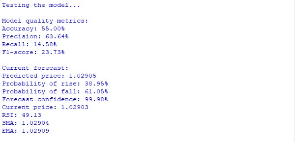
Key performance metrics

• Accuracy: 55.00% Moderately exceeds random guessing for the volatile EURUSD market.
• Precision: 63.64% Shows good reliability of the signals generated by the system - almost two thirds of the forecasts are correct.
• Recall: 14.58% Low recall indicates that the system is selective and generates signals only when there is high confidence in the forecast. This helps avoid false signals.
• F1-score: 23.73% The F1-score value reflects the balance between precision and recall, confirming the conservative strategy of the system.

Current market forecast

• Current EURUSD price: 1.02903
• Predicted price: 1.02905
• Probability distribution:
  • Growth probability: 38.95%
  • Fall probability: 61.05%
• Forecast confidence: 99.98%

The system predicts a moderate upward move with high confidence despite the prevailing probability of a decline. This may indicate a period of short-term correction within the overall downward trend.

Technical Indicators

• RSI: 49.13 (close to neutral zone, indicates no clear overbought or oversold conditions)
• SMA: 1.02904
• EMA: 1.02909
• Trend: neutral (current price is near moving average levels)

Summary

The system exhibits the following key characteristics:

1. Consistent accuracy above random guessing
2. High selectivity in signal generation (63.64% accurate predictions)
3. Ability to quantify the confidence and probabilities of different scenarios
4. A comprehensive analysis of the market situation, taking into account both technical indicators and more complex patterns

This conservative approach, which prioritizes the quality of signals over their quantity, makes the system a potentially effective tool for real trading.

Integrating machine learning metrics and quantum algorithms: Thoughts and first attempts

The combination of quantum computing and machine learning opens new horizons. In our experiment, MinMaxScaler from sklearn is used to normalize the data before quantum encoding it, converting market data into quantum angles.

The system combines machine learning metrics (accuracy, precision, recall, F1-score) with quantum measurements. With an accuracy of 60%, it captures patterns that are inaccessible to classic algorithms, demonstrating caution and selectivity, like an experienced trader.

The future of such systems is the integration of sophisticated preprocessing methods, such as autoencoders and transformers, for deeper data analysis. Quantum algorithms can become a filter for classical models or vice versa, adapting to market conditions.

Our experiment proves that the synergy of quantum and classical methods is not a choice, but a path to the next breakthrough in algorithmic trading.

How I started writing my first quantum neural network - classifier

When I started experimenting with quantum computing in trading, I decided to go beyond simple quantum circuits and create a hybrid system that combines quantum computing with classical machine learning methods. The idea seemed promising. I was going to use quantum states to encode market information, and then train a conventional classifier on that data.

The system turned out to be quite complex. It is based on an 8-qubit quantum circuit that converts market data into quantum states through a series of quantum gates. Each piece of price history is encoded into rotation angles of ry gates, and entanglement between qubits is created using cx gates. This allows the system to capture complex non-linear relationships in the data.

To enhance the predictive ability, I added a set of classic binary indicators: price direction, momentum, volumes, moving average convergence/divergence, volatility, RSI and Bollinger bands. Each indicator generates binary signals which are then combined with quantum features.

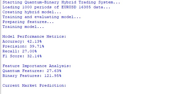
import numpy as np
import MetaTrader5 as mt5
import pandas as pd
from datetime import datetime, timedelta
from qiskit import QuantumCircuit, transpile, QuantumRegister, ClassicalRegister
from qiskit_aer import AerSimulator
from sklearn.preprocessing import MinMaxScaler, StandardScaler
from sklearn.metrics import accuracy_score, precision_score, recall_score, f1_score
from sklearn.model_selection import train_test_split
from catboost import CatBoostClassifier
import warnings
warnings.filterwarnings('ignore')

class MT5DataLoader:
    def __init__(self, symbol="EURUSD", timeframe=mt5.TIMEFRAME_H1):
        if not mt5.initialize():
            raise Exception("MetaTrader5 initialization failed")
        
        self.symbol = symbol
        self.timeframe = timeframe
    
    def get_historical_data(self, lookback_bars=1000):
        current_time = datetime.now()
        rates = mt5.copy_rates_from(self.symbol, self.timeframe, current_time, lookback_bars)
        
        if rates is None:
            raise Exception(f"Failed to get data for {self.symbol}")
            
        df = pd.DataFrame(rates)
        df['time'] = pd.to_datetime(df['time'], unit='s')
        return df

class BinaryPatternGenerator:
    def __init__(self, df, lookback=10):
        self.df = df
        self.lookback = lookback
        
    def direction_encoding(self):
        return (self.df['close'] > self.df['close'].shift(1)).astype(int)
        
    def momentum_encoding(self, threshold=0.0001):
        returns = self.df['close'].pct_change()
        return (returns.abs() > threshold).astype(int)
        
    def volume_encoding(self):
        return (self.df['tick_volume'] > self.df['tick_volume'].rolling(self.lookback).mean()).astype(int)
        
    def convergence_encoding(self):
        ma_fast = self.df['close'].rolling(5).mean()
        ma_slow = self.df['close'].rolling(20).mean()
        return (ma_fast > ma_slow).astype(int)
        
    def volatility_encoding(self):
        volatility = self.df['high'] - self.df['low']
        avg_volatility = volatility.rolling(20).mean()
        return (volatility > avg_volatility).astype(int)
        
    def rsi_encoding(self, period=14, threshold=50):
        delta = self.df['close'].diff()
        gain = (delta.where(delta > 0, 0)).ewm(alpha=1/period).mean()
        loss = (-delta.where(delta < 0, 0)).ewm(alpha=1/period).mean()
        rs = gain / loss
        rsi = 100 - (100 / (1 + rs))
        return (rsi > threshold).astype(int)
        
    def bollinger_encoding(self, window=20):
        ma = self.df['close'].rolling(window=window).mean()
        std = self.df['close'].rolling(window=window).std()
        upper = ma + (std * 2)
        lower = ma - (std * 2)
        return ((self.df['close'] - lower)/(upper - lower) > 0.5).astype(int)
        
    def get_all_patterns(self):
        patterns = {
            'direction': self.direction_encoding(),
            'momentum': self.momentum_encoding(),
            'volume': self.volume_encoding(),
            'convergence': self.convergence_encoding(),
            'volatility': self.volatility_encoding(),
            'rsi': self.rsi_encoding(),
            'bollinger': self.bollinger_encoding()
        }
        return patterns

class QuantumFeatureGenerator:
    def __init__(self, num_qubits=8):
        self.num_qubits = num_qubits
        self.simulator = AerSimulator()
        self.scaler = MinMaxScaler()
        
    def create_quantum_circuit(self, market_data, current_price):
        qr = QuantumRegister(self.num_qubits, 'qr')
        cr = ClassicalRegister(self.num_qubits, 'cr')
        qc = QuantumCircuit(qr, cr)
        
        # Normalize data
        scaled_data = self.scaler.fit_transform(market_data.reshape(-1, 1)).flatten()
        
        # Create superposition
        for i in range(self.num_qubits):
            qc.h(qr[i])
        
        # Apply market data as phases
        for i in range(min(len(scaled_data), self.num_qubits)):
            angle = float(scaled_data[i] * np.pi)
            qc.ry(angle, qr[i])
        
        # Create entanglement
        for i in range(self.num_qubits - 1):
            qc.cx(qr[i], qr[i + 1])
        
        # Add the current price
        price_angle = float((current_price % 0.01) * 100 * np.pi)
        qc.ry(price_angle, qr[0])
        
        qc.measure(qr, cr)
        return qc
        
    def get_quantum_features(self, market_data, current_price):
        qc = self.create_quantum_circuit(market_data, current_price)
        compiled_circuit = transpile(qc, self.simulator, optimization_level=3)
        job = self.simulator.run(compiled_circuit, shots=2000)
        result = job.result()
        counts = result.get_counts()
        
        # Create a vector of quantum features
        feature_vector = np.zeros(2**self.num_qubits)
        total_shots = sum(counts.values())
        
        for bitstring, count in counts.items():
            index = int(bitstring, 2)
            feature_vector[index] = count / total_shots
            
        return feature_vector


class HybridQuantumBinaryPredictor:
    def __init__(self, num_qubits=8, lookback=10, forecast_window=5):
        self.num_qubits = num_qubits
        self.lookback = lookback
        self.forecast_window = forecast_window
        self.quantum_generator = QuantumFeatureGenerator(num_qubits)
        self.model = CatBoostClassifier(
            iterations=500,
            learning_rate=0.03,
            depth=6,
            loss_function='Logloss',
            verbose=False
        )
        
    def prepare_features(self, df):
        """Prepare hybrid features"""
        pattern_generator = BinaryPatternGenerator(df, self.lookback)
        binary_patterns = pattern_generator.get_all_patterns()
        
        features = []
        labels = []
        
        # Fill NaN in binary patterns
        for key in binary_patterns:
            binary_patterns[key] = binary_patterns[key].fillna(0)
        
        for i in range(self.lookback, len(df) - self.forecast_window):
            try:
                # Quantum features
                market_data = df['close'].iloc[i-self.lookback:i].values
                current_price = df['close'].iloc[i]
                quantum_features = self.quantum_generator.get_quantum_features(market_data, current_price)
                
                # Binary features
                binary_vector = []
                for key in binary_patterns:
                    window = binary_patterns[key].iloc[i-self.lookback:i].values
                    binary_vector.extend([
                        sum(window),  # Total number of signals
                        window[-1],   # Last signal
                        sum(window[-3:])  # Last 3 signals
                    ])
                
                # Technical indicators
                rsi = binary_patterns['rsi'].iloc[i]
                bollinger = binary_patterns['bollinger'].iloc[i]
                momentum = binary_patterns['momentum'].iloc[i]
                
                # Combine all features
                feature_vector = np.concatenate([
                    quantum_features,
                    binary_vector,
                    [rsi, bollinger, momentum]
                ])
                
                # Label: price movement direction
                future_price = df['close'].iloc[i + self.forecast_window]
                current_price = df['close'].iloc[i]
                label = 1 if future_price > current_price else 0
                
                features.append(feature_vector)
                labels.append(label)
                
            except Exception as e:
                print(f"Error at index {i}: {str(e)}")
                continue
        
        return np.array(features), np.array(labels)
    
    def train(self, df):
        """Train hybrid model"""
        print("Preparing features...")
        X, y = self.prepare_features(df)
        
        # Split into training and test samples
        split_point = int(len(X) * 0.8)
        X_train, X_test = X[:split_point], X[split_point:]
        y_train, y_test = y[:split_point], y[split_point:]
        
        print("Training model...")
        self.model.fit(X_train, y_train, eval_set=(X_test, y_test))
        
        # Model evaluation
        predictions = self.model.predict(X_test)
        probas = self.model.predict_proba(X_test)
        
        # Calculate metrics
        metrics = {
            'accuracy': accuracy_score(y_test, predictions),
            'precision': precision_score(y_test, predictions),
            'recall': recall_score(y_test, predictions),
            'f1': f1_score(y_test, predictions)
        }
        
        # Feature importance analysis
        feature_importance = self.model.feature_importances_
        quantum_importance = np.mean(feature_importance[:2**self.num_qubits])
        binary_importance = np.mean(feature_importance[2**self.num_qubits:])
        
        metrics.update({
            'quantum_importance': quantum_importance,
            'binary_importance': binary_importance,
            'test_predictions': predictions,
            'test_probas': probas,
            'test_actual': y_test
        })
        
        return metrics
    
    def predict_next(self, df):
        """Next movement forecast"""
        X, _ = self.prepare_features(df)
        if len(X) > 0:
            last_features = X[-1].reshape(1, -1)
            prediction_proba = self.model.predict_proba(last_features)[0]
            prediction = self.model.predict(last_features)[0]
            
            return {
                'direction': 'UP' if prediction == 1 else 'DOWN',
                'probability_up': prediction_proba[1],
                'probability_down': prediction_proba[0],
                'confidence': max(prediction_proba)
            }
        return None

def test_hybrid_model(symbol="EURUSD", timeframe=mt5.TIMEFRAME_H1, periods=1000):
    """Full test of the hybrid model"""
    try:
        # MT5 initialization
        if not mt5.initialize():
            raise Exception("Failed to initialize MT5")
        
        # Download data
        print(f"Loading {periods} periods of {symbol} {timeframe} data...")
        loader = MT5DataLoader(symbol, timeframe)
        df = loader.get_historical_data(periods)
        
        # Create and train model
        print("Creating hybrid model...")
        model = HybridQuantumBinaryPredictor()
        
        # Training and assessment
        print("Training and evaluating model...")
        metrics = model.train(df)
        
        # Output results
        print("\nModel Performance Metrics:")
        print(f"Accuracy: {metrics['accuracy']:.2%}")
        print(f"Precision: {metrics['precision']:.2%}")
        print(f"Recall: {metrics['recall']:.2%}")
        print(f"F1 Score: {metrics['f1']:.2%}")
        
        print("\nFeature Importance Analysis:")
        print(f"Quantum Features: {metrics['quantum_importance']:.2%}")
        print(f"Binary Features: {metrics['binary_importance']:.2%}")
        
        # Current forecast
        print("\nCurrent Market Prediction:")
        prediction = model.predict_next(df)
        if prediction:
            print(f"Predicted Direction: {prediction['direction']}")
            print(f"Up Probability: {prediction['probability_up']:.2%}")
            print(f"Down Probability: {prediction['probability_down']:.2%}")
            print(f"Confidence: {prediction['confidence']:.2%}")
        
        return model, metrics
        
    finally:
        mt5.shutdown()

if __name__ == "__main__":
    print("Starting Quantum-Binary Hybrid Trading System...")
    model, metrics = test_hybrid_model()
    print("\nSystem test completed.")

The initial results were sobering. On EURUSD H1, the system accuracy was only 42.13%, which is even worse than random guessing. Precision of 39.71% and recall of 27% indicate that the model is significantly wrong in its predictions. The F1 score of 32.14% confirms the overall weakness of the forecasts.

The analysis of feature importance turned out to be particularly interesting. Quantum features contributed only 27.63% to the overall predictive power of the model, while binary features showed the significance of 121.95%. This suggests that either the quantum part of the system is not picking up important patterns in the data, or the quantum encoding method itself requires serious improvement.

But these results are not discouraging - on the contrary, they point to specific areas for improvement. Perhaps, it is worth changing the quantum encoding circuit, increasing or decreasing the number of qubits and experimenting with other quantum gates. Or maybe the problem lies in how quantum and conventional features integrate with each other.

The experiment showed that creating an efficient quantum-classical hybrid system is not simply a matter of combining the two approaches. It requires a deep understanding of both quantum computing and the specifics of financial markets. This is just the first step in a long journey of research and optimization.

In future iterations, I plan to significantly rework the quantum part of the system, possibly adding more complex quantum transformations and improving the way market information is encoded into quantum states. It is also worth experimenting with different ways of combining quantum and classical features to find the optimal balance between them.

Conclusion

I thought combining quantum computing with technical analysis was a great idea. You know, like in the movies: take a cool technology, add a little machine learning magic, and voila - a money printing press is ready! The reality proved me wrong.

My "brilliant" quantum classifier barely scraped together 42% accuracy. This is worse than flipping a coin! And you know what is funniest? All these fancy quantum features that I spent weeks working on brought only 27% benefit. And the good old technical indicators that I added "just in case" shot up by 122%.

I was especially excited when I started grasping quantum data encoding. Just imagine - we take ordinary price movements and turn them into quantum states! It sounds like science fiction, but it really works. Although, not quite as I would like it to work.

My quantum classifier is still more like a broken calculator than a trading system of the future. But I do not give up. Because somewhere out there, in this strange world of quantum states and market patterns, there is something really worthwhile hiding. And I intend to find it, even if I have to rewrite the entire code from scratch.

In the meantime... I am getting back to my qubits. Still, the ordinary "quantum" scheme showed some results. Better than guessing... But I have a couple of ideas on how to make this thing work. And I will definitely tell you about them.

Programs used in the article

File	File contents
Quant_Predict_p_1.py	Classical quantum prediction with an attempt to discover the prototype
Quant_Neural_Link.py	Draft version of the quantum neural network
Quant_ML_Model.py	Draft version of the quantum machine learning model