Neural networks made easy (Part 28): Policy gradient algorithm

MetaTrader 5 — Trading systems | 16 November 2022, 14:13

5 647

Dmitriy Gizlyk

Introduction

We continue studying different reinforcement learning methods. In the previous article, we got acquainted with the Deep Q-Learning method. This method approximates the action utility function using a neural network. As a result, we get a tool for predicting the expected reward when performing a specific action in a particular system state. After that, the agent performs an action based on the policy and the amount of the expected reward. We have not explicitly discussed the use of policy but have assumed the choice of the action with the highest expected reward. This follows from the Bellman formula and the overall goal of reinforcement learning, which is to maximize the rewards for the analyzed session.

Also notice, when studying reinforcement learning methods, we never mentioned model overfitting. In fact, if you look at the reinforcement learning model, then the goal of the agent is to learn the environment as best as possible. The better the agent knows the environment, the better it performs.

But when we deal with a changing environment, which is the market, then sometimes you realize that there is no limit to its variability. There are no two identical states in the market. Even when there are similar states, we can get to absolutely opposite states at the next step.

Approximation of the Q-function only provides the expected average reward, without taking into account the spread of values and the probability of a positive reward. The use of a greedy strategy with the choice of the maximum reward always gives an unambiguous action selection. On the one hand, this makes the agent work easier. But such a strategy gives the desired result only as long as our agent is not in some kind of confrontation with the environment. In this case, its actions become predictable for the environment, and it can develop steps to counter the agent's actions and change the reward policy. However, the agent will continue to use the previously approximated Q-function, which will no longer correspond to the changed environment.

Such problems can be solved using methods that do not approximate the reward policy of the environment, but they develop their own behavioral strategy. One of such methods is policy gradient, which we will discuss in this article.

1. Policy gradient application features

When starting learning reinforcement learning methods, we mentioned that the Agent interacts with the environment and performs actions in accordance with its strategy. This results in a transition from one state to another. For each transition, the agent receives a certain reward from the environment. By the reward value, the agent can evaluate the usefulness of the action taken. The policy gradient method implies the development of an agent behavior strategy.

Of course, we do not explicitly set the agent's strategy, as can be seen in DQN. We only make an assumption about the existence of a certain mathematical function of the policy P, which evaluates the current state of the environment and returns the best action the agent takes. This approach eliminates all the difficulties of approximating the Q-function, as well as the need to specify an explicit agent behavior policy, such as the selection of an action with a maximum expected reward (greedy strategy).

Of course, everything has its price. Instead of approximating the Q function we will have to approximate the P function of our agent's policy. This article will focus on the stochastic policy gradient method. It assumes that our policy function, when assessing the current state of the environment, returns the probability distribution of receiving a positive reward when performing the corresponding action.

At the same time, we assume that our agent's actions are distributed evenly. To select a specific action, the agent can simply sample a value from a normal distribution with given probabilities. Of course, it is possible to use a greedy strategy and select a highest-probability action. But it is sampling that adds variability to the agent's behavior. A greater probability increases the frequency of selecting this particular action.

Remember, earlier, when in reinforcement learning of models, we introduced a hyperparameter that is responsible for the balance of exploration and exploitation. Now, when using the stochastic policy gradient method, this balance is regulated by the model in the learning process through the use of probability-based agent actions sampling. At the beginning of the model training, the probabilities of all actions are almost equal. This enables the most complete exploration of the environment. In the process of studying the environment, the probabilities of actions leading to the maximized profitability are increased. The probability of selecting other actions is reduced. Thus, the balance of exploration and exploitation changes in favor of selecting the most profitable actions, which allows building a strategy with maximum profitability.

To approximate the agent's policy P-function, we will use a neural network. Since we need to determine the best action of the agent based on the initial data of the current environment state, this task can be considered as a classification problem. Each action is a separate class of initial states. As mentioned earlier, the neural layer output should provide a probabilistic representation which particular state the environment state belongs to.

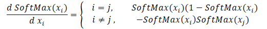
The probabilistic representation imposes some restrictions on the resulting value. The results must be normalized in the range between 0% and 100%. The sum of all probabilities must be equal to 100%. In machine learning, it is common to use fractions of one instead of percentages. Therefore, the range of values should be from 0 to 1, while the sum of all values should be 1. This result can be obtained by using the SoftMax function which has the following mathematical formula.

SoftMax

We have already seen this function before, when studying data clustering methods. But when studying unsupervised learning methods, we looked into similarities in source data to determine the class. This time, we will distribute the environment states into actions (classes) depending on the reward received. The SoftMax function fully satisfies these requirements. It enables the complete transfer of the neural network operation results into the domain of probabilities and is differentiable throughout the values. Which is very important for the model training.

2. Policy model learning principles

Now let's talk about the principles of training the policy function approximation model. When training the DQN model on each new state, the environment returned a reward. We trained the model to predict the expected reward with minimal error. Which was not much different from the previously used supervised learning approaches.

When approximating the agent's policy P-function on each new state, we also receive a reward from the environment. But we want to predict the best action and not the reward. The reward sign can only show the impact of the current action on the result. We will train the model to increase the probability of choosing an action with a positive reward and decrease the probability of choosing an action with a negative reward.

But we train the model to predict the probability. As mentioned above, the values of the predicted probabilities are limited to the range from 0 to 1. But this is not comparable to the reward received, which can be both positive and negative. Let's use the following logic here. Since we need to maximize the probability of choosing actions with a positive reward, the target value for such actions we be 1. The model error will be defined as the deviation of the predicted probability of an action from 1. The use of the deviation/variance allows exploiting the already built gradient descent method to train the policy function approximation model, since by minimizing the variance from 1 we maximize the probability of choosing an action with a positive reward.

Please note the choice of the loss function for the model. Here we can also get back to supervised learning methods and remember that the cross entropy function is used for classification problems.

LogLoss

where p(y) are the true values of the distribution, and p(y') are the predicted values of the model.

The use of the logarithm is also of great importance for predicting successive events. We know from probability theory that the probability of two successive events occurring is equal to the product of the event probabilities. The following is true for logarithms

This allows transferring from the product of the probabilities to the sum of their logarithms. This will make the model training more stable.

Similar to DQN training, to receive the rewards, the agent passes a session with fixed parameters. Save the states, actions and rewards to the buffer. Then execute the backpropagation pass using the accumulated data.

Note that since we don't have an action utility function, we replace it with the sum of the values obtained during the session pass. For each state, the value of the Q-function is the sum of subsequent rewards up to the end of the session.

Model training is repeated until the desired error level or the maximum number of training sessions is reached.

3. Implementing model training

We have discussed the theoretical aspects, and now let's move on to its implementation using MQL5. Let's start with the SoftMax function. We have not implemented it as an activation function earlier due to its operation specifics. So, to avoid making cardinal changes to previously created objects, we will implement it as a separate layer of the model.

3.1 Implementing SoftMax

So, create a new class CNeuronSoftMaxOCL derived from the base class of neurons CNeuronBaseOCL.

class CNeuronSoftMaxOCL    :  public CNeuronBaseOCL
  {
protected:
   virtual bool      feedForward(CNeuronBaseOCL *NeuronOCL) override;
   virtual bool      updateInputWeights(CNeuronBaseOCL *NeuronOCL) override { return true; }

public:
                     CNeuronSoftMaxOCL(void) {};
                    ~CNeuronSoftMaxOCL(void) {};
   virtual bool      calcInputGradients(CNeuronBaseOCL *NeuronOCL);   
   virtual bool      calcOutputGradients(CArrayFloat *Target, float error) override;
   //---
   virtual int       Type(void) override  const   {  return defNeuronSoftMaxOCL; }
  };

The new class does not require the creation of separate buffers. Moreover, it does not use all of the buffers of the parent class, which we will talk about a little later. That is why the constructor and the destructor are empty. For the same reason, there is no need to override our class initialization method. Actually, we will only need to override the feedForward feed forward pass and the calcOutputGradients error gradient methods.

Also, since we us a new loss function, it is necessary to override the model error and gradient calculation method calcOutputGradients.

And, of course, we will override the class identification method Type.

Let's start by implementing the feed forward pass process. Again, all computational operations will be performed in multi-thread mode using OpenCL. So, let's create the new kernel SoftMax_FeedForward in OpenCL. In the kernel parameters, we will pass pointers to the initial data and results buffers, along with the buffer size. Function calculation does not require any additional parameters.

In the kernel body, define the thread identifier, which serves as a pointer to the corresponding element of the initial data and results array. Since this is an implementation of the activation function, the sizes of the initial data buffer and the results buffer are equal. Therefore, the pointer to the elements of these two buffers will be the same.

__kernel void SoftMax_FeedForward(__global float *inputs,
                                  __global float *outputs,
                                  const ulong total)
  {
   uint i = (uint)get_global_id(0);
   uint l = (uint)get_local_id(0);
   uint ls = min((uint)get_local_size(0), (uint)256);
//---
   __local float temp[256];

Note that to calculate the SoftMax function, it is necessary to determine sum of the exponential values of all elements of the input data buffer. It wouldn't be good to repeat the calculations of this value at each thread. Furthermore, it would be good to distribute the parameter calculation process between multiple threads. However, here we encounter a problem of synchronizing the work of several threads and exchanging data between them. OpenCL technology does not allow sending data from one thread to another. But it allows creating common variables and arrays in local memory within separate workgroups. To synchronize the work of threads within the workgroup, there is a specialized function barrier(CLK_LOCAL_MEM_FENCE). This is what we are going to use.

Therefore, along with the defining of the thread ID in the global task space, we will define the thread ID in the group. Also, we will declare an array in the local memory. It will be used to exchange data between the workgroup threads when calculating the total sum of exponential values.

The difficult part here is that OpenCL does not allow the use of dynamic arrays in local memory. Therefore, the array size should be determined at the kernel creation stage. This size limits the number of threads used to sum exponential values.

The process of summing exponential values consists of 2 successive loops. In the body of the first loop, each thread participating in the summation process will iterate through the entire vector of initial values with a step equal to the number of summation threads and will collect its part of the sum of exponential values. Thus, we will evenly distribute the entire summation process among all threads. Each of them will store its value in the corresponding element of the local array.

   uint count = 0;
   if(l < 256)
      do
        {
         uint shift = count * ls + l;
         temp[l] = (count > 0 ? temp[l] : 0) + (count * ls + l < total ? exp(inputs[shift]) : 0);
         count++;
        }
      while((count * ls + l) < total);
   barrier(CLK_LOCAL_MEM_FENCE);

At this stage, we synchronize the threads after the loop iterations have completed.

Next, we need to collect the sum of all elements of the local array into a single value. This will be implemented in the second loop. Here we divide the size of the local array in half and add the values in pairs. Each operation related of adding two values will be performed by a separate thread. After that, repeat the loop iterations: dividing the number of elements in half and adding the elements in pairs. The loop iterations are repeated until we get the total sum of the values in the array element with index 0.

   count = ls;
   do
     {
      count = (count + 1) / 2;
      if(l < 256)
         temp[l] += (l < count && (l + count) < total ? temp[l + count] : 0);
      barrier(CLK_LOCAL_MEM_FENCE);
     }
   while(count > 1);

As you can see, each new iteration of the loop can only start after the operations of all participating threads have completed. Therefore, the synchronization is performed after each iteration of the loop.

Please note here that the OpenCL architecture provides only full synchronization of threads. So, all elements in the workgroup must reach the relevant 'barrier' operator. Otherwise, the program will freeze. Therefore, when organizing the program, you need to be very careful about thread synchronization points. It is not recommended to implement them in the bodies of conditional operators, when the program algorithm allows at least one thread to bypass the synchronization points.

Once the iterations of the above loops have completed, we get the sum of all the exponential values of the original data and can complete the data normalization process. To do this, we will create another loop, in which the initial data buffer will be filled with the corresponding values.

   float sum = temp[0];
   if(sum != 0)
     {
      count = 0;
      while((count * ls + l) < total)
        {
         uint shift = count * ls + l;
         outputs[shift] = exp(inputs[shift]) / (sum + 1e-37f);
         count++;
        }
     }
  }

This concludes operations with the feed forward kernel. Next, we move on to creating the backpropagation kernels.

We will start with the creation with the backpropagation kernels by distributing the gradient through the softmax function. Pay attention that the main feature of this function is the normalization of the sum of all result values to 1. Therefore, a change in only one value at the activation function input leads to recalculation of all values of the result vector. Similarly, when propagating the error gradient, each element of the input data must receive its share of the error from each element of the result vector. The mathematical formula for the influence of each initial data element on the result is presented below. This is what we will implement in the kernel SoftMax_HiddenGradient.

In parameters, the kernel receives pointers to 3 data buffers: results after a feed-forward pass, gradients from a previous layer or from a loss function. Also, it receives the gradient buffer of the previous layer, in which we will write the results of this kernel.

In the kernel body, define the thread identifier and the total number of running threads. They will point to an array element to record the result of the current thread and the buffer sizes.

Next, we need to prepare two private variables. Copy the value of the corresponding element of the feed-forward result vector into one of them. The second one should be declared to collects the current thread operation results. We use private variables due to the specific architecture of OpenCL devices. Accessing private variables is much faster than similar operations with buffers in global memory. So, this approach improves the overall performance of the kernel.

Then we loop through all results elements to collect the error gradient from according to the above formula. After completing the loop operations, pass the accumulated gradient value to the corresponding element of the gradient buffer of the previous layer and close the kernel.

__kernel void SoftMax_HiddenGradient(__global float* outputs,
                                    __global float* output_gr,
                                    __global float* input_gr)
  {
   size_t i = get_global_id(0);
   size_t outputs_total = get_global_size(0);
   float output = outputs[i];
   float result = 0;
   for(int j = 0; j < outputs_total; j++)
      result += outputs[j] * output_gr[j] * ((float)(i == j ? 1 : 0) - output);
   input_gr[i] = result;
  }

There is the last kernel — the one for determining the error gradient of the loss function SoftMax_OutputGradient. In this article, we use LogLoss as the loss function.

LogLoss

Since the gradients are distributed to the elements of the corresponding action, the derivative will also be calculated element by element. This allows splitting the error gradient across threads. From the school mathematics course, we know that the derivative of the logarithm is equal to the ratio of 1 to the argument of the function. Therefore, the derivative of the loss function will be as follows.

now, we need to implement the above mathematical formula in the OpenCL program kernel. Its code is quite simple and takes only two lines.

__kernel void SoftMax_OutputGradient(__global float* outputs,
                                     __global float* targets,
                                     __global float* output_gr)
  {
   size_t i = get_global_id(0);
   output_gr[i] = -targets[i] / (outputs[i] + 1e-37f);
  }

This completes operation on the OpenCL program side. Now, we can move to working with the main program. We need to add constants for working with new kernels, add a declaration of the new kernels and create methods for calling them.

#define def_k_SoftMax_FeedForward         36
#define def_k_softmaxff_inputs            0
#define def_k_softmaxff_outputs           1
#define def_k_softmaxff_total             2
//---
#define def_k_SoftMax_HiddenGradient      37
#define def_k_softmaxhg_outputs           0
#define def_k_softmaxhg_output_gr         1
#define def_k_softmaxhg_input_gr          2
//---
#define def_k_SoftMax_OutputGradient      38
#define def_k_softmaxog_outputs           0
#define def_k_softmaxog_targets           1
#define def_k_softmaxog_output_gr         2

Kernel calling methods completely repeat the previously used algorithms of similar methods. Their full code can be found in the attachment.

The missing SoftMax function is now ready, and we can start move on to the Expert Advisor, where we will implement and train the policy gradient model.

3.2 Building an EA to train the model

To train the agent policy function approximation model, we will create a new Expert Advisor in the REINFORCE.mq5 file. The basic functionality is inherited from Q-learning.mq5 which we created in the last article to train the DQN model. However, unlike the DQN model, the new Expert Advisor will only use one neural network. For the correct implementation of the algorithm, we need to create three stacks: environment states, actions taken, and rewards received.

CNet                StudyNet;
CArrayObj           States;
vectorf             vActions;
vectorf             vRewards;

The EA's external parameters are slightly changed, as required by the algorithm.

input int                  SesionSize =  24 * 22;
input int                  Iterations = 1000;
input double               DiscountFactor =   0.999;

The EA initialization method is almost the same. We have only added stack initialization to accumulate actions performed and rewards received.

   if(!vActions.Resize(SesionSize) ||
      !vRewards.Resize(SesionSize))
      return INIT_FAILED;

The training process is implemented in the Train function. Let us consider it in more detail.

As usual, at the beginning of the function we determine the training sample range in accordance with the given external parameters.

void Train(void)
  {
//---
   MqlDateTime start_time;
   TimeCurrent(start_time);
   start_time.year -= StudyPeriod;
   if(start_time.year <= 0)
      start_time.year = 1900;
   datetime st_time = StructToTime(start_time);

After determining the training period, load the training sample.

   int bars = CopyRates(Symb.Name(), TimeFrame, st_time, TimeCurrent(), Rates);
   if(!RSI.BufferResize(bars) || !CCI.BufferResize(bars) || !ATR.BufferResize(bars) || !MACD.BufferResize(bars))
     {
      ExpertRemove();
      return;
     }
   if(!ArraySetAsSeries(Rates, true))
     {
      ExpertRemove();
      return;
     }
//---
   RSI.Refresh();
   CCI.Refresh();
   ATR.Refresh();
   MACD.Refresh();
//---
   int total = bars - (int)(HistoryBars + 2 * SesionSize);

The above operations do not differ from those used in earlier EAs. This is followed by a system of model training loops. The system implements the main approaches to model training.

The outer loop is responsible for iterating over the model training sessions. At the beginning of the cycle, we randomly determine the session beginning bar in the general pool of the loaded history.

   CBufferFloat* State;
   for(int iter = 0; (iter < Iterations && !IsStopped()); iter ++)
     {
      int error_code;
      int shift = (int)(fmin(fabs(Math::MathRandomNormal(0,1,error_code)),1) * (total) + SesionSize);
      States.Clear();

Then implement a loop in which our agent, step by step, completely goes through the session. In the body of the loop, first fill the buffer of the current system state with historical data for the analyzed period. A similar operation was performed when training previous models, before each direct pass.

      for(int batch = 0; batch < SesionSize; batch++)
        {
         int i = shift - batch;
         State = new CBufferFloat();
         if(!State)
           {
            ExpertRemove();
            return;
           }
         int r = i + (int)HistoryBars;
         if(r > bars)
            continue;
         for(int b = 0; b < (int)HistoryBars; b++)
           {
            int bar_t = r - b;
            float open = (float)Rates[bar_t].open;
            TimeToStruct(Rates[bar_t].time, sTime);
            float rsi = (float)RSI.Main(bar_t);
            float cci = (float)CCI.Main(bar_t);
            float atr = (float)ATR.Main(bar_t);
            float macd = (float)MACD.Main(bar_t);
            float sign = (float)MACD.Signal(bar_t);
            if(rsi == EMPTY_VALUE || cci == EMPTY_VALUE || atr == EMPTY_VALUE || macd == EMPTY_VALUE || sign == EMPTY_VALUE)
               continue;
            //---
            if(!State.Add((float)Rates[bar_t].close - open) || !State.Add((float)Rates[bar_t].high - open) ||
               !State.Add((float)Rates[bar_t].low - open) || !State.Add((float)Rates[bar_t].tick_volume / 1000.0f) ||
               !State.Add(sTime.hour) || !State.Add(sTime.day_of_week) || !State.Add(sTime.mon) ||
               !State.Add(rsi) || !State.Add(cci) || !State.Add(atr) || !State.Add(macd) || !State.Add(sign))
               break;
           }

Next, implement the model feed forward pass.

         if(IsStopped())
           {
            ExpertRemove();
            return;
           }
         if(State.Total() < (int)HistoryBars * 12)
            continue;
         if(!StudyNet.feedForward(GetPointer(State), 12, true))
           {
            ExpertRemove();
            return;
           }

Based on the results of the feed forward pass, we get a probability distribution of actions and also sample the next action from the normal distribution, taking into account the obtained probability distribution. Sampling is performed by a separate function GetAction; the probability distribution is passed in its parameters.

         StudyNet.getResults(TempData);
         int action = GetAction(TempData);
         if(action < 0)
           {
            ExpertRemove();
            return;
           }

After sampling the action, determine the reward for the selected action based on the size of the next candlestick. The reward policy is the one we used in the previous article.

         double reward = Rates[i - 1].close - Rates[i - 1].open;
         switch(action)
           {
            case 0:
               if(reward < 0)
                  reward *= -2;
               break;
            case 1:
               if(reward > 0)
                  reward *= -2;
               else
                  reward *= -1;
               break;
            default:
               reward = -fabs(reward);
               break;
           }

Save the entire sample to the stack. Please note that the states and actions are simply added to the stack. But the rewards are saved considering the discount factor. Therefore, at the design step, we need to determine how to discount the rewards. There are two options for discounting. We can discount early rewards by giving more value to later rewards. This approach is often used when the agent receives intermediate rewards while going through the session. But the main task of the agent is to get to the end of the session, where it will receive the maximum reward.

The second approach is reversed: more weight is given to the first rewards. Later rewards are then discounted. This option is acceptable when we aim for the maximum and fastest reward. I used the second approach, because it is important to immediately get the maximum profit, and not wait in loss while the market reverses after the deal.

And one moment. After completing the session pass, we have to calculate the cumulative reward from each state until the end of the session. MQL5 vector operations allow calculating only the direct cumulative sum. Therefore, we will simply store all reward values into a vector in reverse order. After the end of the loop, use a vector operation to calculate the cumulative sum.

         if(!States.Add(State))
           {
            ExpertRemove();
            return;
           }
         vActions[batch] = (float)action;
         vRewards[SessionSize - batch - 1] = (float)(reward * pow(DiscountFactor, (double)batch));
         vProbs[SessionSize - batch - 1] = TempData.At(action);
         //---
        }

After saving the data, move on to the next iteration of the loop. Thus, we collect data for the entire session.

After all iterations of the loop, calculate the total reward for the session considering the discount, the vector of cumulative rewards from each state until the end of the session, and the value of the loss function.

Also, save the current model, but only if the maximum reward is updated.

      float cum_reward = vRewards.Sum();
      vRewards = vRewards.CumSum();
      vRewards = vRewards / fmax(vRewards.Max(), fabs(vRewards.Min()));
      float loss = (vRewards * MathLog(vProbs) * (-1)).Sum();
      if(MaxProfit < cum_reward)
        {
         if(!StudyNet.Save(FileName + ".nnw", loss, 0, 0, Rates[shift - SessionSize].time, false))
            return;
         MaxProfit = cum_reward;
        }

Now that we have the values of the rewards along the agent's session path, we can implement a training loop for the policy function model. This will be implemented in another loop. In this loop, we extract the environment states from our buffer and execute the model feed forward pass. This is necessary to restore all the internal values of the model for the corresponding state of the environment.

After that, prepare a vector of reference values for the current state of the environment. As you remember, we maximize the probability of choosing an action with the positive reward and minimize the probabilities of others. Therefore, if after action execution we receive a positive value, fill the vector of reference probabilities with zero values. And only for the executed action set the probability to 1. If a negative reward is returned, fill the vector of reference probabilities with ones. Zero is set for the executed action in this case.

      for(int batch = 0; batch < SessionSize; batch++)
        {
         State = States.At(batch);
         if(!StudyNet.feedForward(State))
           {
            ExpertRemove();
            return;
           }
         if((vRewards[SessionSize - batch - 1] >= 0 ?
             (!TempData.BufferInit(Actions, 0) || !TempData.Update((int)vActions[batch], 1)) :
             (!TempData.BufferInit(Actions, 1) || !TempData.Update((int)vActions[batch], 0))
            ))
           {
            ExpertRemove();
            return;
           }
         if(!StudyNet.backProp(TempData))
           {
            ExpertRemove();
            return;
           }
        }

Next, run the backpropagation pass to update the model weights. Repeat the iterations for all saved environment states.

After completing all iterations of the loop, print a message to the log and move on to the next session.

      PrintFormat("Iteration %d, Cummulative reward %.5f, loss %.5f", iter, cum_reward, loss);
     }
   Comment("");
//---
   ExpertRemove();
  }

Do not forget to check the operation result at each step. After the successful completion of all iterations, exit the function and generate a terminal close event. The full EA code can be found in the attachment.

Also note that to approximate the policy function of our model, we used a neural network with an architecture similar to the Q-function training from the last article. Moreover, we use the trained model from the last article and replaced the decision block in it by adding SoftMax as the last layer of the neural network to normalize the data.

The model training process is completely similar to training any other model. There are a lot of examples in each article within this series. So, to summarize the work done, I decided to deviate from the usual article format. Instead, set us look at how the trained models run in the strategy tester.

4. Testing the trained model in the Strategy Tester

In the previous article, we trained a DQN model. In this article, we created and trained a policy gradient model. I propose to create testing Expert Advisors, using which we can look at how the models perform in the strategy tester. So, let's create two EAs: Q-learning-test.mq5 and REINFORCE-test.mq5. The names reflect the models tested by each EA.

The EAs have the same structure. Therefore, let's take a look at one of them. Anyway, the full code of both EAs can be found in the attachment.

The new EA "REINFORCE-test.mq5" is constructed on the basis of the REINFORCE.mq5 EA discussed above. But since the EA will not train the model, the Train function has been removed. The basic functionality has been moved to the OnTick function which processes every new tick event.

The trained model evaluates the environment states based on closed candlestick. Therefore, in the body of the OnTick function, check the opening of a new candle. The remaining operations of the function will be performed only if a new candlestick appears.

//+------------------------------------------------------------------+
//| Expert tick function                                             |
//+------------------------------------------------------------------+
void OnTick()
  {
   if(lastBar >= iTime(Symb.Name(), TimeFrame, 0))
      return;

When a new candlestick appears, load the latest historical data and fill in the system state description buffer.

   int bars = CopyRates(Symb.Name(), TimeFrame, 0, HistoryBars+1, Rates);
   if(!ArraySetAsSeries(Rates, true))
      return;
   RSI.Refresh();
   CCI.Refresh();
   ATR.Refresh();
   MACD.Refresh();
//---
   State1.Clear();
   for(int b = 0; b < (int)HistoryBars; b++)
     {
      int bar_t = (int)HistoryBars - b;
      float open = (float)Rates[bar_t].open;
      TimeToStruct(Rates[bar_t].time, sTime);
      float rsi = (float)RSI.Main(bar_t);
      float cci = (float)CCI.Main(bar_t);
      float atr = (float)ATR.Main(bar_t);
      float macd = (float)MACD.Main(bar_t);
      float sign = (float)MACD.Signal(bar_t);
      if(rsi == EMPTY_VALUE || cci == EMPTY_VALUE || atr == EMPTY_VALUE || macd == EMPTY_VALUE || sign == EMPTY_VALUE)
         continue;
      //---
      if(!State1.Add((float)Rates[bar_t].close - open) || !State1.Add((float)Rates[bar_t].high - open) ||
         !State1.Add((float)Rates[bar_t].low - open) || !State1.Add((float)Rates[bar_t].tick_volume / 1000.0f) ||
         !State1.Add(sTime.hour) || !State1.Add(sTime.day_of_week) || !State1.Add(sTime.mon) ||
         !State1.Add(rsi) || !State1.Add(cci) || !State1.Add(atr) || !State1.Add(macd) || !State1.Add(sign))
         break;
     }

Next, check if the data is filled correctly and implement the model feed forward pass.

   if(State1.Total() < (int)(HistoryBars * 12))
      return;
   if(!StudyNet.feedForward(GetPointer(State1), 12, true))
      return;
   StudyNet.getResults(TempData);
   if(!TempData)
     return;

As a result of the feed forward pass, we get a probability distribution of possible actions, from which we sample a random action.

   lastBar = Rates[0].time;
   int action = GetAction(TempData);
   delete TempData;

Next, the selected action should be executed. But before moving on to opening a new deal, check if there are already open positions. To do this, define 2 flags: Buy and Sell. When declaring variables, set them to false.

After that implement a loop through all values. If an open position for the analyzed symbol is found, change the value of the corresponding flag.

   bool Buy = false;
   bool Sell = false;
   for(int i = 0; i < PositionsTotal(); i++)
     {
      if(PositionGetSymbol(i) != Symb.Name())
         continue;
      switch((ENUM_POSITION_TYPE)PositionGetInteger(POSITION_TYPE))
        {
         case POSITION_TYPE_BUY:
            Buy = true;
            break;
         case POSITION_TYPE_SELL:
            Sell = true;
            break;
        }
     }

This is followed by the trading block. Here we use the 'switch' statement to branch the block algorithm depending on the action being taken. If it is opening a new position, check the flags of open positions. If there is an open position in the relevant direction, simply leave it in the market and wait for the opening of a new candlestick.

If, at the time of making the decision, an open opposite position is found, first close the open position and only then open a new one.

   switch(action)
     {
      case 0:
         if(!Buy)
           {
            if((Sell && !Trade.PositionClose(Symb.Name())) ||
               !Trade.Buy(Symb.LotsMin(), Symb.Name()))
              {
               lastBar = 0;
               return;
              }
           }
         break;
      case 1:
         if(!Sell)
           {
            if((Buy && !Trade.PositionClose(Symb.Name())) ||
               !Trade.Sell(Symb.LotsMin(), Symb.Name()))
              {
               lastBar = 0;
               return;
              }
           }
         break;
      case 2:
         if(Buy || Sell)
            if(!Trade.PositionClose(Symb.Name()))
              {
               lastBar = 0;
               return;
              }
         break;
     }
//---
  }

If the agent needs to close all positions, call the function for closing positions for the current symbol. The function is only called if there is at least one open position.

Do not forget to control the results at each step.

The full EA code can be found in the attachment.

The first tested model was DQN. And it shows an unexpected surprise. The model generated a profit. But it executed only one trading operation, which was open throughout the test. The symbol chart with the executed deal is shown below.

Testing DQN

By evaluating the deal on the symbol chart, you can see that the model clearly identified the global trend and opened a deal in its direction. The deal is profitable, but the question is whether the model will be able to close such a deal in time? In fact, we trained the model using historical data for the last 2 years. For all the 2 years, the market has been dominated by a bearish trend for the analyzed instrument. That is why we wonder if the model can close the deal in time.

When using the greedy strategy, the policy gradient model gives similar results. Remember, when we started studying reinforcement learning methods, I repeatedly emphasized the importance of the right choice of reward policy. So, I decided to experiment with the reward policy. In particular, in order to exclude too long holding of losing position, I decided to increase the penalties for unprofitable positions. For this, I additionally trained the policy gradient model using the new reward policy. After some experiments with the model hyperparameters, I managed to achieve 60% profitable operations. The testing graph is shown below.

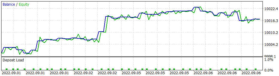
The average position holding time is 1 hour 40 minutes.

Conclusion

In this article, we discussed studied another algorithms of reinforcement learning methods. We created and trained a model using the policy gradient method.

Unlike other articles in this series, in this article we trained and tested the models in the strategy tester. Based on testing results, we can conclude that the models can generate signals for executing profitable trading operations. At the same time, I would like to emphasize once again, that it is important to select the right reward policy and loss function to achieve the desired result.

List of references

Programs used in the article

#	Name	Type	Description
1	REINFORCE.mq5	EA	An Expert Advisor to train the model
2	REINFORCE-test.mq5	EA	An Expert Advisor to test the model in the Strategy Tester
1	Q-learning-test.mq5	EA	An Expert Advisor to test the DQN model in the Strategy Tester
2	NeuroNet.mqh	Class library	Library for creating neural network models
3	NeuroNet.cl	Code Base	OpenCL program code library to create neural network models

…

Translated from Russian by MetaQuotes Ltd.
Original article: https://www.mql5.com/ru/articles/11392

Attached files |

Download ZIP

MQL5.zip (73.44 KB)

Warning: All rights to these materials are reserved by MetaQuotes Ltd. Copying or reprinting of these materials in whole or in part is prohibited.