Neural Networks in Trading: Enhancing Transformer Efficiency by Reducing Sharpness (SAMformer)

Introduction

Multivariate time series forecasting is a classical machine learning task that involves analyzing time series data to predict future trends based on historical patterns. It is a particularly challenging problem due to feature correlations and long-term temporal dependencies. This learning problem is common in real-world applications where observations are collected sequentially (e.g., medical data, electricity consumption, stock prices).

Recently, Transformer-based architectures have achieved breakthrough performance in natural language processing and computer vision tasks. Transformers are especially effective when working with sequential data, making them a natural fit for time series forecasting. However, state-of-the-art multivariate time series forecasting is still often achieved using simpler MLP-based models.

Recent studies applying Transformers to time series data have primarily focused on optimizing attention mechanisms to reduce quadratic computational costs or decomposing time series to better capture their underlying patterns. However, the authors of the paper "SAMformer: Unlocking the Potential of Transformers in Time Series Forecasting with Sharpness-Aware Minimization and Channel-Wise Attention" highlight a critical issue: the training instability of Transformers in the absence of large-scale data.

In both computer vision and NLP, it has been observed that attention matrices can suffer from entropy collapse or rank collapse. Several approaches have been proposed to mitigate these problems. Yet, in time series forecasting, it remains an open question how to train Transformer architectures effectively without overfitting. The authors aim to demonstrate that addressing training instability can significantly improve Transformer performance in long-term multivariate forecasting, contrary to previously established ideas about their limitations.

1. The SAMformer algorithm

The focus is on long-term forecasting in a multivariate system, given a D-dimensional time series of length L (the lookback window). The input data is represented as a matrix 𝐗 ∈ RD×L. The objective is to predict the next H values (the forecast horizon), denoted as 𝐘 ∈ RD×H. Assuming access to a training set consisting of N observations, the goal is to train a forecasting model f𝝎: RD×L→RD×L with parameters 𝝎 that minimizes the mean squared error (MSE) on the training data.

Recent findings show that Transformers perform on par with simple linear neural networks trained to directly project input data into forecast values. To investigate this phenomenon, the SAMformer framework adopts a generative model simulating a synthetic regression task that mimics the time series forecasting setup. The authors use a linear model to generate time series continuations from random input data, adding a small amount of noise to the output. This process produced 15,000 input-output pairs, split into 10,000 for training and 5,000 for validation.

Leveraging this generative approach, the SAMformer authors design a Transformer architecture capable of addressing the forecasting task efficiently and without unnecessary complexity. To achieve this, they simplify the conventional Transformer encoder by retaining only the Self-Attention block followed by a residual connection. Instead of a FeedForward block, a linear layer is directly used for forecasting the subsequent values.

It is important to note that the SAMformer framework employs channel-wise attention, which simplifies the task and reduces the risk of over-parameterization, as the attention matrix becomes significantly smaller due to L>D. Moreover, channel-wise attention is more appropriate here since the data generation follows an identification process.

To understand the role of attention in solving this task, the authors propose a model named Random Transformer. In this model, only the forecasting layer is optimized, while the parameters of the Self-Attention block are fixed at random initialization during training. This effectively forces the Transformer to behave as a linear model. A comparison of the local minima obtained by these two models. optimized using the Adam method, with an Oracle model (which corresponds to the least squares solution) is presented in the figure below (as visualized in the original paper).

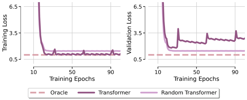
The first surprising finding is that neither Transformer model is able to recover the linear dependency of the synthetic regression task, highlighting that optimization, even in such a simple architecture with favorable design, demonstrates a clear lack of generalization. This observation holds true across different optimizers and learning rate settings. From this, the SAMformer authors conclude that the limited generalization capabilities of Transformers primarily stem from training difficulties within the attention module.

To better understand this phenomenon, the SAMformer authors visualized the attention matrices at various training epochs and found that the attention matrix closely resembled an identity matrix immediately after the first epoch and changed very little thereafter, especially as the Softmax function amplified the differences between attention values. This behavior reveals the onset of entropy collapse in attention, resulting in a full-rank attention matrix, which the authors identify as one of the causes of the Transformer's training rigidity.

The SAMformer authors also observed a relationship between entropy collapse and the sharpness of the Transformer's loss landscape. Compared to the Random Transformer, the standard Transformer converges to a sharper minimum and exhibits significantly lower entropy (as the attention weights in the Random Transformer are fixed at initialization, its entropy remains constant throughout training). These pathological patterns suggest that Transformers underperform due to the dual effect of entropy collapse and sharp loss landscapes during training.

Recent studies have confirmed that the loss landscape of Transformers is indeed sharper than that of other architectures. This may help explain the training instability and lower performance of Transformers, especially when trained on smaller datasets.

To address these challenges and improve generalization and training stability, the SAMformer authors explore two approaches. The first involves Sharpness-Aware Minimization (SAM), which modifies the training objective as follows:

where ρ>0 is a hyperparameter, and 𝝎 represents the model parameters.

The second approach introduces reparameterization of all weight matrices using spectral normalization along with an additional trainable scalar known as σReparam.

The results highlight the success of the proposed solution in achieving the desired outcome. Remarkably, this is accomplished using SAM alone, as the σReparam method fails to approach optimal performance, despite increasing the attention matrix entropy. Furthermore, the sharpness achieved under SAM is several orders of magnitude lower than that of a standard Transformer, while the attention entropy under SAM remains comparable to that of the baseline Transformer, with only a modest increase in the later stages of training. This indicates that entropy collapse is benign in this scenario.

The SAMformer framework further incorporates Reversible Instance Normalization (RevIN). This method has proven effective in handling distribution shifts between training and testing data in time series. As demonstrated by the research above, the model is optimized using SAM, guiding it toward flatter local minima. Overall, this results in a simplified Transformer model with a single encoder block, as shown in the figure below (original visualization from the authors).

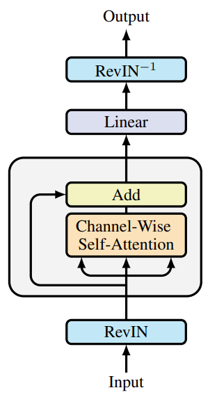
It is important to emphasize that SAMformer retains channel-wise attention, represented by a D×D matrix, unlike spatial (or temporal) attention, which typically relies on a L×L matrix in other models. This design offers two key advantages:

• Permutation invariance of features, eliminating the need for positional encoding, which is usually applied prior to the attention layer;
• Reduced computational time and memory complexity, as D≤L in most real-world datasets.

Channel-wise attention learns the average influence of each feature on the others across all time steps.

2. Implementation in MQL5

After covering the theoretical aspects of the SAMformer framework, we now move on to its practical implementation using MQL5. At this point, it is important to define exactly what we intend to implement in our models and how. Let's take a closer look at the components suggested by the SAMformer authors:

• Trimming the Transformer encoder down to the Self-Attention block with a residual connection;
• Channel-wise attention;
• Reversible normalization (RevIN);
• SAM optimization.

The encoder trimming is an interesting aspect. However, in practical terms, its main value lies in reducing the number of trainable parameters. Functionally, the model behavior is unaffected by how we label neural layers as part of the Encoder's FeedForward block or as a forecasting layer placed after attention, as done in the original framework.

To implement channel-wise attention, it's sufficient to transpose the input data before feeding it into the attention block. This step requires no structural changes to the model.

We're already familiar with Reversible Instance Normalization (RevIN). The remaining task is to implement SAM optimization, which operates by seeking parameter sets that lie in neighborhoods with uniformly low loss values.

The SAM optimization algorithm involves several steps. First, a feed-forward pass is performed to compute the loss gradients with respect to model parameters. These gradients are then normalized and added to the current parameters, scaled by a sharpness coefficient. A second feed-forward pass is performed using these perturbed parameters, and the new gradients are computed. Then, we restore the original weights by subtracting the previously added perturbation. And finally update the parameters using a standard optimizer — SGD or Adam. The SAMformer authors suggest using the latter.

An important detail is that the SAMformer authors normalize gradients across the entire model. This can be computationally intensive. This raises the relevance of reducing the number of model parameters. As a result, trimming internal layers and reducing the number of attention heads becomes a practical necessity. Which is what the SAMformer framework authors did.

In our implementation, however, we diverge slightly: we perform gradient normalization at the level of individual neural layers. Furthermore, we normalize gradients separately for each parameter group that contributes to a single neuron's output. We begin this implementation by developing new kernels on the OpenCL side of the program.

2.1 Extending the OpenCL Program

As you may have noticed from our previous work, we primarily rely on two types of neural layers: fully connected and convolutional. All our attention modules are built using convolutional layers, applied without overlap to analyze and transform individual elements in the sequence. Therefore, we chose to enhance these two layer types with SAM optimization. On the OpenCL side, we will develop two kernels: one for gradient normalization, and another for generating the perturbed weights ω+ε.

We begin by creating a kernel for the fully connected layer CalcEpsilonWeights. This kernel receives pointers to four data buffers and a sharpness dispersion coefficient. Three buffers hold the input data, while the fourth is designated for storing the output results. 

__kernel void CalcEpsilonWeights(__global const float *matrix_w,
                                 __global const float *matrix_g,
                                 __global const float *matrix_i,
                                 __global float *matrix_epsw,
                                 const float rho
                                )
  {
   const size_t inp = get_local_id(0);
   const size_t inputs = get_local_size(0) - 1;
   const size_t out = get_global_id(1);

We plan to invoke this kernel in a two-dimensional task space, grouping threads by the first dimension. Inside the kernel body, we immediately identify the current execution thread across all dimensions of the task space.

Next, we declare a local memory array on the device to facilitate data exchange between threads within the same work group.

   __local float temp[LOCAL_ARRAY_SIZE];
   const int ls = min((int)inputs, (int)LOCAL_ARRAY_SIZE);

In the following step, we compute the gradient of the error for each analyzed element as the product of corresponding elements in the input and output gradient buffers. We then scale this result by the absolute value of the associated parameter. This will increase the influence of parameters that contribute more significantly to the layer's output.

   const int shift_w = out * (inputs + 1) + inp;
   const float w =IsNaNOrInf(matrix_w[shift_w],0);
   float grad = fabs(w) * IsNaNOrInf(matrix_g[out],0) * (inputs == inp ? 1.0f : IsNaNOrInf(matrix_i[inp],0));

Finally, we compute the L2 norm of the resulting gradients. This involves summing the squares of the computed values within the work group, using the local memory array and two reduction loops, following the approach used in our previous implementations.

   const int local_shift = inp % ls;
   for(int i = 0; i <= inputs; i += ls)
     {
      if(i <= inp && inp < (i + ls))
         temp[local_shift] = (i == 0 ? 0 : temp[local_shift]) + IsNaNOrInf(grad * grad,0);
      barrier(CLK_LOCAL_MEM_FENCE);
     }
//---
   int count = ls;
   do
     {
      count = (count + 1) / 2;
      if(inp < count)
         temp[inp] += ((inp + count) < inputs ? IsNaNOrInf(temp[inp + count],0) : 0);
      if(inp + count < inputs)
         temp[inp + count] = 0;
      barrier(CLK_LOCAL_MEM_FENCE);
     }
   while(count > 1);

The square root of the accumulated sum represents the L2 norm of the gradients. Using this value, we compute the adjusted parameter value.

   float norm = sqrt(IsNaNOrInf(temp[0],0));
   float epsw = IsNaNOrInf(w * w * grad * rho / (norm + 1.2e-7), w);
//---
   matrix_epsw[shift_w] = epsw;
  }

We then save the resulting value in the corresponding element of the global result buffer.

A similar approach is used to construct the CalcEpsilonWeightsConv kernel, which performs the initial parameter adjustment for convolutional layers. However, as you know, convolutional layers have their own characteristics. They typically contain fewer parameters, but each parameter interacts with multiple elements of the input data layer and contributes to the values of several elements in the result buffer. As a result, the gradient for each parameter is computed by aggregating its influence from multiple elements of the output buffer.

This convolution-specific behavior also affects the kernel parameters. Here, two additional constants appear, defining the size of the input sequence and the stride of the input window.

__kernel void CalcEpsilonWeightsConv(__global const float *matrix_w,
                                     __global const float *matrix_g,
                                     __global const float *matrix_i,
                                     __global float *matrix_epsw,
                                     const int inputs,
                                     const float rho,
                                     const int step
                                    )
  {
//---
   const size_t inp = get_local_id(0);
   const size_t window_in = get_local_size(0) - 1;
   const size_t out = get_global_id(1);
   const size_t window_out = get_global_size(1);
   const size_t v = get_global_id(2);
   const size_t variables = get_global_size(2);

We also extend the task space to three dimensions. The first dimension corresponds to the input data window, expanded with an offset. The second dimension represents the number of convolutional filters. The third dimension accounts for the number of independent input sequences. As before, we group operation threads by the first dimension into workgroups.

Inside the kernel, we identify the current execution thread across all task-space dimensions. We then initialize a local memory array within the OpenCL context to facilitate inter-thread communication within the workgroup.

   __local float temp[LOCAL_ARRAY_SIZE];
   const int ls = min((int)(window_in + 1), (int)LOCAL_ARRAY_SIZE);

Next, we calculate the number of elements per filter in the output buffer and determine the corresponding offsets in the data buffers.

   const int shift_w = (out + v * window_out) * (window_in + 1) + inp;
   const int total = (inputs - window_in + step - 1) / step;
   const int shift_out = v * total * window_out + out;
   const int shift_in = v * inputs + inp;
   const float w = IsNaNOrInf(matrix_w[shift_w], 0);

At this point, we also store the current value of the parameter being analyzed in a local variable. This optimization reduces the number of accesses to global memory in later steps.

In the next stage, we collect the gradient contribution from all elements of the output buffer that were influenced by the parameter under analysis.

   float grad = 0;
   for(int t = 0; t < total; t++)
     {
      if(inp != window_in && (inp + t * step) >= inputs)
         break;
      float g = IsNaNOrInf(matrix_g[t * window_out + shift_out],0);
      float i = IsNaNOrInf(inp == window_in ? 1.0f : matrix_i[t * step + shift_in],0);
      grad += IsNaNOrInf(g * i,0);
     }

We then scale the collected gradient by the absolute value of the parameter.

   grad *= fabs(w);

Following this, we apply the previously described two-stage reduction algorithm to sum the squares of the gradients within the workgroup.

   const int local_shift = inp % ls;
   for(int i = 0; i <= inputs; i += ls)
     {
      if(i <= inp && inp < (i + ls))
         temp[local_shift] = (i == 0 ? 0 : temp[local_shift]) + IsNaNOrInf(grad * grad,0);
      barrier(CLK_LOCAL_MEM_FENCE);
     }
//---
   int count = ls;
   do
     {
      count = (count + 1) / 2;
      if(inp < count)
         temp[inp] += ((inp + count) < inputs ? IsNaNOrInf(temp[inp + count],0) : 0);
      if(inp + count < inputs)
         temp[inp + count] = 0;
      barrier(CLK_LOCAL_MEM_FENCE);
     }
   while(count > 1);

The square root of the resulting sum yields the desired L2 norm of the error gradients.

   float norm = sqrt(IsNaNOrInf(temp[0],0));
   float epsw = IsNaNOrInf(w * w * grad * rho / (norm + 1.2e-7),w);
//---
   matrix_epsw[shift_w] = epsw;
  }

We then compute the adjusted parameter value and store it in the appropriate element of the result buffer.

This concludes our work on the OpenCL-side implementation. The full code can be found in the attached file.

2.2 Fully Connected Layer with SAM Optimization

After completing the work on the OpenCL side, we move on to our library implementation, where we create the object for a fully connected layer with integrated SAM optimization - CNeuronBaseSAMOCL. The structure of the new class is shown below.

class CNeuronBaseSAMOCL  :  public CNeuronBaseOCL
  {
protected:
   float             fRho;
   CBufferFloat      cWeightsSAM;
   //---
   virtual bool      calcEpsilonWeights(CNeuronBaseSAMOCL *NeuronOCL);
   virtual bool      feedForwardSAM(CNeuronBaseSAMOCL *NeuronOCL);
   virtual bool      updateInputWeights(CNeuronBaseOCL *NeuronOCL);

public:
                     CNeuronBaseSAMOCL(void) {};
                    ~CNeuronBaseSAMOCL(void) {};
   //---
   virtual bool      Init(uint numOutputs, uint myIndex, COpenCLMy *open_cl, 
                          uint numNeurons, float rho, 
                          ENUM_OPTIMIZATION optimization_type, uint batch);
   //---
   virtual bool      Save(int const file_handle);
   virtual bool      Load(int const file_handle);
   //---
   virtual int       Type(void)        const    {  return defNeuronBaseSAMOCL;      }
   virtual int       Activation(void)  const    {  return (fRho == 0 ? (int)None : (int)activation);   }
   virtual int       getWeightsSAMIndex(void)   {  return cWeightsSAM.GetIndex();   }
   //---
   virtual CLayerDescription* GetLayerInfo(void);
   virtual void      SetOpenCL(COpenCLMy *obj);
  };

As you can see from the structure, the main functionality is inherited from the base fully connected layer. Basically, this class is a copy of the base layer, with the parameter update method overridden to incorporate SAM optimization logic.

That said, we've added a wrapper method calcEpsilonWeights to interface with the corresponding kernel described earlier, and we’ve also created a modified version of the forward pass method that uses an altered weight buffer named feedForwardSAM.

It's worth noting that in the original SAMformer framework, the authors applied ε to the model parameters, then subtracted it afterward to restore the original state. We approached this differently. We store the perturbed parameters in a separate buffer. This allowed us to bypass the ε subtraction step, thus reducing total execution time. But first things first.

The buffer for the perturbed model parameters is declared statically, allowing us to leave the constructor and destructor empty. Initialization of all declared and inherited objects is performed in the Init method.

bool CNeuronBaseSAMOCL::Init(uint numOutputs, uint myIndex, COpenCLMy *open_cl, uint numNeurons, 
                             float rho, ENUM_OPTIMIZATION optimization_type, uint batch)
  {
   if(!CNeuronBaseOCL::Init(numOutputs, myIndex, open_cl, numNeurons, optimization_type, batch))
      return false;

In the method parameters, we receive the main constants that determine the architecture of the created object. Inside the method, we immediately call the Init method of the parent class, which implements validation and initialization of inherited components.

Once the parent method completes successfully, we store the sharpness radius coefficient in an internal variable.

   fRho = fabs(rho);
   if(fRho == 0 || !Weights)
      return true;

Next, we check the value of the sharpness coefficient and the presence of a parameter matrix. If the coefficient is equal to "0" or if the parameter matrix is absent (meaning the layer has no outgoing connections), the method exits successfully. Otherwise, we need to create a buffer for the alternative parameters. Structurally it is identical to the main weight buffer, but initialized with zero values at this stage.

   if(!cWeightsSAM.BufferInit(Weights.Total(), 0) ||
      !cWeightsSAM.BufferCreate(OpenCL))
      return false;
//---
   return true;
  }

This completes the method.

We suggest you review the wrapper methods for enqueuing OpenCL kernels on your own. Their code is provided in the attachment. Let's move on to the parameter update method: updateInputWeights.

bool CNeuronBaseSAMOCL::updateInputWeights(CNeuronBaseOCL *NeuronOCL)
  {
   if(!NeuronOCL)
      return false;
   if(NeuronOCL.Type() != Type() || fRho == 0)
      return CNeuronBaseOCL::updateInputWeights(NeuronOCL);

This method receives a pointer to the input data object, as usual. We immediately validate the pointer, as any further operation would result in critical errors if the pointer is invalid.

We also verify the type of the input data object, as it is important in this context. Additionally, the sharpness coefficient must be greater than "0". Otherwise, the SAM logic degenerates into standard optimization. Then we call the relevant method of the parent class.

Once these checks are passed, we proceed to the execution of operations of the SAM method. Recall that the SAM algorithm involves a full feed-forward and backpropagation pass, distributing the error gradients after perturbing the parameters with ε. However, earlier we established that our SAM implementation operates at the level of a single layer. This raises the question: where do we get the target values for each layer?

At first glance, the solution seems straightforward - simply sum the last feed-forward pass result with the error gradient. But there's a caveat. When the gradient is passed from the subsequent layer, it is typically adjusted by the derivative of the activation function. Thus, simple summation would distort the result. One option would be to implement a mechanism that reverses the gradient correction based on the activation derivative. However, we found a simpler and more efficient solution: we override the activation function return method, so that if the sharpness coefficient is zero, the method returns None. This way, we receive the raw error gradient from the next layer, unmodified by the activation derivative. Thus, we can add the feed-forward pass result and the error gradient. The sum of these two gives us the effective target for the layer being analyzed.

   if(!SumAndNormilize(Gradient, Output, Gradient, 1, false, 0, 0, 0, 1))
      return false;

Next we call the wrapper method to get the adjusted model parameters.

   if(!calcEpsilonWeights(NeuronOCL))
      return false;

And we perform a feed-forward pass with perturbed parameters.

   if(!feedForwardSAM(NeuronOCL))
      return false;

At this point, the error gradient buffer contains the target values, while the result buffer holds the output produced by the perturbed parameters. To determine the deviation between these values, we simply call the parent class method for calculating the deviation from target outputs.

   float error = 1;
   if(!calcOutputGradients(Gradient, error))
      return false;

Now, we only need to update the model parameters based on the updated error gradient. This is done by calling the corresponding method from the parent class.

   return CNeuronBaseOCL::updateInputWeights(NeuronOCL);
  }

A few words should be said about file operation methods. To save disk space, we chose not to save the perturbed weight buffer cWeightsSAM. Keeping its data has no practical value since this buffer is only relevant during parameter updates. It is overwritten on each call. Thus, the size of saved data increased by only one float element (the coefficient).

bool CNeuronBaseSAMOCL::Save(const int file_handle)
  {
   if(!CNeuronBaseOCL::Save(file_handle))
      return false;
   if(FileWriteFloat(file_handle, fRho) < INT_VALUE)
      return false;
//---
   return true;
  }

On the other hand, the cWeightsSAM buffer is still necessary for performing the required functionality. Its size is critical, as it must be sufficient to hold all parameters of the current layer. Therefore, we need to recreate it when loading a previously saved model. In the data loading method, we first call the equivalent method from the base class.

bool CNeuronBaseSAMOCL::Load(const int file_handle)
  {
   if(!CNeuronBaseOCL::Load(file_handle))
      return false;

Next, we check for file content beyond the base structure, and if present, we read in the sharpness coefficient.

   if(FileIsEnding(file_handle))
      return false;
   fRho = FileReadFloat(file_handle);

We then verify that the sharpness coefficient is non-zero and ensure that a valid parameter matrix exists (note: its pointer may be invalid in the case of layers with no outgoing connections).

   if(fRho == 0 || !Weights)
      return true;

If either check fails, parameter optimization degrades into basic methods, and there's no need to recreate a buffer of adjusted parameters. Therefore, we exit the method successfully.

It should be noted that failing this check is critical for SAM optimization, but not for model operation as a whole. Therefore, the program continues using the base optimization methods.

If buffer creation is necessary, we first clear the existing buffer. We intentionally skip checking the result of the clear operation. This is because situations are possible where the buffer may not yet exist when loading. 

   cWeightsSAM.BufferFree();

We then initialize a new buffer of appropriate size with zero values and create its OpenCL copy.

   if(!cWeightsSAM.BufferInit(Weights.Total(), 0) ||
      !cWeightsSAM.BufferCreate(OpenCL))
      return false;
//---
   return true;
  }

This time, we do validate the execution of these operations, since their success is critical for further operation of the model. Upon completion, we return the operation status to the calling function.

This concludes our discussion of the implementation of the fully connected layer with SAM optimization support (CNeuronBaseSAMOCL). The full source code for this class and its methods can be found in the provided attachment.

Unfortunately, we have reached the volume limit of this article but we haven't yet completed the work. In the next article, we will continue the implementation and look at the convolutional layer with the implementation of the SAM functionality. Let's We will also look at the application of the proposed technologies in the Transformer architecture and, of course, test the performance of the proposed approaches on real historical data.

Conclusion

SAMformer provides an effective solution to the core drawbacks of Transformer models in long-term forecasting of multivariate time series, such as training complexity and poor generalization on small datasets. By using a shallow architecture and sharpness-aware optimization, SAMformer not only avoids poor local minima but also outperforms state-of-the-art methods. Furthermore, it uses fewer parameters. The results presented by the authors confirm its potential as a universal tool for time series tasks.

In the practical part of our article, we have built our vision of the proposed approaches using MQL5. But our work is still ongoing. In the next article, we will evaluate the practical value of the proposed approaches for solving our problems.

References

SAMformer: Unlocking the Potential of Transformers in Time Series Forecasting with Sharpness-Aware Minimization and Channel-Wise Attention

Sharpness-Aware Minimization for Efficiently Improving Generalization

Other articles from this series

Programs used in the article

#	Name	Type	Description
1	Research.mq5	Expert Advisor	Expert Advisor for collecting examples
2	ResearchRealORL.mq5	Expert Advisor	Expert Advisor for collecting examples using the Real-ORL method
3	Study.mq5	Expert Advisor	Model training Expert Advisor
4	StudyEncoder.mq5	Expert Advisor	Encode training EA
5	Test.mq5	Expert Advisor	Model testing Expert Advisor
6	Trajectory.mqh	Class library	System state description structure
7	NeuroNet.mqh	Class library	A library of classes for creating a neural network
8	NeuroNet.cl	Library	OpenCL program code library