Neural Networks in Trading: Hyperbolic Latent Diffusion Model (HypDiff)

Introduction

Graphs contain the diversity and significance in the topological structures of raw data. These topological features often reflect underlying physical principles and development patterns. Traditional random graph models based on classical graph theory rely heavily on artificial heuristics to design algorithms for specific topologies and lack the flexibility to effectively model diverse and complex graph structures. To address these limitations, numerous deep learning models for graph generation have been developed. Probabilistic diffusion models with denoising capabilities have shown strong performance and potential, particularly in visualization tasks.

However, due to the irregular and non-Euclidean nature of graph structures, applying diffusion models in this context presents two major limitations:

1. High Computational Complexity. Graph generation inherently involves processing discrete, sparse, and other non-Euclidean topological features. The Gaussian noise perturbation used in vanilla diffusion models is not well-suited for discrete data. As a result, discrete graph diffusion models typically exhibit high temporal and spatial complexity due to structural sparsity. Furthermore, such models rely on continuous Gaussian noise processes to generate fully connected, noisy graphs, which often leads to a loss of structural information and the topological properties underlying it.
2. Anisotropy of Non-Euclidean Structures. Unlike data with regular structure, the embeddings of graph nodes in non-Euclidean space are anisotropic within continuous latent space. When node embeddings are mapped into Euclidean space, they exhibit pronounced anisotropy along specific directions. An isotropic diffusion process in latent space tends to treat this anisotropic structural information as noise, leading to its loss during the denoising stage.

Hyperbolic geometric space has been widely recognized as an ideal continuous manifold for representing discrete tree-like or hierarchical structures and is employed in various graph learning tasks. The authors of the paper "Hyperbolic Geometric Latent Diffusion Model for Graph Generation" claim that hyperbolic geometry has great potential for addressing the issue of non-Euclidean structural anisotropy in latent diffusion processes for graphs. In hyperbolic space, the distribution of node embeddings tends to be globally isotropic. Meanwhile, anisotropy is preserved locally. Moreover, hyperbolic geometry unifies angular and radial measurements in polar coordinates, offering geometric dimensions with physical semantics and interpretability. Notably, hyperbolic geometry can furnish latent space with geometric priors that reflect the intrinsic structure of graphs.

Based on these insights, the authors aim to design a suitable latent space grounded in hyperbolic geometry to enable an efficient diffusion process over non-Euclidean structures for graph generation, preserving topological integrity. In doing so, they try to solve two core problems:

1. The additive nature of continuous Gaussian distributions is undefined in hyperbolic latent space.
2. Developing an effective anisotropic diffusion process tailored to non-Euclidean structures.

To overcome these problems, the authors propose a Hyperbolic Latent Diffusion Model (HypDiff). For the problem of Gaussian distribution additivity in hyperbolic space, a diffusion process based on radial measures is introduced. Additionally, angular constraints are applied to limit anisotropic noise, thereby preserving structural priors and guiding the diffusion model toward finer structural details within the graph.

1. The HypDiff Algorithm

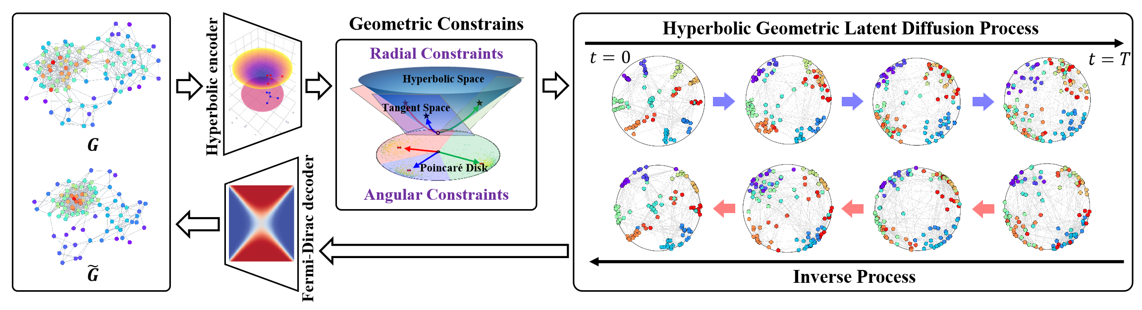
The Hyperbolic Latent Diffusion Model (HypDiff) addresses two key challenges in graph generation. It leverages hyperbolic geometry to abstract the implicit hierarchy of graph nodes and introduces two geometric constraints to preserve essential topological properties. The authors employ a two-stage training strategy. First, they train a hyperbolic autoencoder to obtain pre-trained node embeddings, and second, they train a hyperbolic geometric latent diffusion process.

The initial step involves embedding the graph data 𝒢 = (𝐗, A) into a low-dimensional hyperbolic space, which improves the latent diffusion process of the graph.

The proposed hyperbolic autoencoder comprises a hyperbolic geometric encoder and a Fermi-Dirac decoder. The encoder maps the graph 𝒢 = (𝐗, A) into a hyperbolic geometric space to obtain an appropriate hyperbolic representation, while the Fermi-Dirac decoder reconstructs the representation back into the graph data domain. The hyperbolic manifold ℍᵈ Hd and its tangent space 𝒯x can be interconverted via exponential and logarithmic maps. Multi-layer perceptrons (MLPs) or graph neural networks (GNNs) can be used to operate on these exponential/logarithmic representations. In their implementation, the authors use Hyperbolic Graph Convolutional Networks (HGCNs) as the hyperbolic geometric encoder.

Due to the failure of Gaussian distribution additivity in hyperbolic space, traditional Riemannian normal or wrapped normal distributions cannot be directly applied. Instead of diffusing embeddings directly in hyperbolic space, the authors propose using a product space of multiple manifolds. To address this, the authors of HypDiff introduce a novel diffusion process in hyperbolic space. For computational efficiency, the Gaussian distribution of the hyperbolic space is approximated by the Gaussian distribution of the tangent plane 𝒯μ.

Unlike Euclidean space, which supports linear addition, hyperbolic space uses Möbius addition. This poses challenges for manifold-based diffusion. Moreover, isotropic noise rapidly reduces the signal-to-noise ratio, making it difficult to preserve topological information.

Graph anisotropy in latent space inherently carries inductive bias about graph structure. A central problem is identifying the dominant directions of this anisotropy. To tackle this, the authors of the HypDiff method propose a hyperbolic anisotropic diffusion framework. The core idea here is to select a primary diffusion direction (i.e., angle) based on node clustering by similarity. This can effectively segment hyperbolic latent space into multiple sectors. Each cluster's nodes are then projected onto the tangent plane of their centroid for diffusion.

These clusters can be formed using any similarity-based clustering algorithm during preprocessing.

The hyperbolic clustering parameter k ∈ [1, n] defines the number of sectors partitioning the hyperbolic space. The hyperbolic anisotropic diffusion is equivalent to directed diffusion within the Klein model 𝕂c,n with multiple curvatures Ci ∈|k|, approximated as projections onto the set of tangent planes 𝒯𝐨i∈{|k|} at cluster centroids Oi∈{|k|}.

This property elegantly establishes a connection between the HypDiff authors' approximation algorithm and with the multi-curvature Klein model.

The behavior of the proposed algorithm varies based on the value of k. This enables a more flexible and fine-grained representation of anisotropy in hyperbolic geometry, which enhances accuracy and efficiency during both noise injection and model training.

Hyperbolic geometry can naturally and geometrically describe node connectivity during graph growth. A node's popularity can be abstracted through its radial coordinate, while similarity can be expressed via angular distances in hyperbolic space.

The primary objective is to model diffusion with geometric radial growth, aligned with the intrinsic properties of hyperbolic space.

The fundamental reason why standard diffusion models underperform on graphs is the rapid decline in signal-to-noise ratio. In HypDiff, the geodesic direction from each cluster's center to the north pole O is used as the target diffusion direction, guiding the forward diffusion process under geometric constraints.

Following the standard denoising and reverse diffusion modeling procedure, the authors of HypDiff adopt a UNet-based Denoising Diffusion Model (DDM) to train the prediction of X0.

Furthermore, HypDiff authors demonstrate that sampling can be performed jointly in a single tangent space, rather than across multiple tangent spaces of cluster centers, to improve efficiency.

The authors present the visualization of the HypDiff framework below.

2. Implementation in MQL5

After reviewing the theoretical aspects of the HypDiff method, we now move on to the practical part of the article, where we implement our interpretation of the proposed approaches using MQL5. It is worth noting from the outset that the implementation will be quite long and challenging. So, get prepared for the substantial volume of work.

2.1 Extending the OpenCL Program

We begin our practical implementation by modifying our existing OpenCL program. The first step involves projecting the input data into hyperbolic space. During this transformation, it is crucial to consider each position of an element in the sequence, as hyperbolic space combines Euclidean spatial parameters with temporal aspects. Following the original methodology, we apply the Lorentz model. This projection is implemented in the HyperProjection kernel.

__kernel void HyperProjection(__global const float *inputs,
                              __global float *outputs
                             )
  {
   const size_t pos = get_global_id(0);
   const size_t d = get_local_id(1);
   const size_t total = get_global_size(0);
   const size_t dimension = get_local_size(1);

The kernel will receive pointers to data buffers as parameters: the sequence under analysis and the transformation results. The characteristics of these data buffers will be defined through the workload space. The first dimension corresponds to the length of the sequence, while the second dimension specifies the size of the feature vector describing each individual element in the sequence. Work items will be grouped into workgroups based on the final dimension. 

Note that the feature vector for each sequence element will contain 1 additional component.

Next, we declare a local array for data exchange between threads within a workgroup.

   __local float temp[LOCAL_ARRAY_SIZE];
   const int ls = min((int)dimension, (int)LOCAL_ARRAY_SIZE);

We define the offset constants in the data buffers.

   const int shift_in = pos * dimension + d;
   const int shift_out = pos * (dimension + 1) + d + 1;

Let's load the input data from the global buffer into the local elements of the corresponding workflow and calculate the quadratic values. We should also make sure to check the operation execution result.

   float v = inputs[shift_in];
   if(isinf(v) || isnan(v))
      v = 0;
//---
   float v2 = v * v;
   if(isinf(v2) || isnan(v2))
      v2 = 0;

Next, we need to calculate the norm of the input data vector. To do this, we sum the square of its values using our local array. This is because each workgroup thread contains 1 element.

//---
   if(d < ls)
      temp[d] = v2;
   barrier(CLK_LOCAL_MEM_FENCE);
   for(int i = ls; i < (int)dimension; i += ls)
     {
      if(d >= i && d < (i + ls))
         temp[d % ls] += v2;
      barrier(CLK_LOCAL_MEM_FENCE);
     }
//---
   int count = min(ls, (int)dimension);
//---
   do
     {
      count = (count + 1) / 2;
      if(d < count)
         temp[d] += ((d + count) < dimension ? temp[d + count] : 0);
      if(d + count < dimension)
         temp[d + count] = 0;
      barrier(CLK_LOCAL_MEM_FENCE);
     }
   while(count > 1);

It should be noted here that we need the vector norm only to calculate the value of the first element in our vector describing the hyperbolic coordinates of the element of the sequence being analyzed. We move all other elements without changes, but with a shift in position.

   outputs[shift_out] = v;

To avoid extra operations, we determine the value of the first element of the hyperbolic vector only in the first thread of each workgroup.

Here we first calculate the proportion of offset in the analyzed element in the original sequence. And then we subtract the square of the obtained norm value of the initial representation vector calculated above. Finally, we calculate the square root of the obtained value.

   if(d == 0)
     {
      v = ((float)pos) / ((float)total);
      if(isinf(v) || isnan(v))
         v = 0;
      outputs[shift_out - 1] = sqrt(fmax(temp[0] - v * v, 1.2e-07f));
     }
  }

Note that when extracting square roots, we explicitly ensure that only values greater than zero are used. This eliminates the risk of runtime errors and invalid results during computation.

To implement backpropagation algorithms, we will immediately create the HyperProjectionGrad kernel, which implements the error gradient propagation through the previously defined feed-forward operations. Please pay attention to the following two points. First, the position of an element within the sequence is static and non-parametric. This means that no gradient is propagated to it.

Second, the gradient of the remaining elements is propagated through two separate information threads. One is the direct gradient propagation. Simultaneously, all components of the original feature vector were used in computing the vector norm, which in turn determines the first element of the hyperbolic representation. Therefore, each feature must receive a proportionate share of the error gradient from the first element of the hyperbolic vector.

Let us now examine how these approaches are implemented in code. The HyperProjectionGrad kernel takes 3 data buffer pointers as parameters. A new input gradient buffer (inputs_gr) is introduced. The buffer containing the hyperbolic representation of the original sequence is replaced by its corresponding error gradient buffer (outputs_gr).

__kernel void HyperProjectionGrad(__global const float *inputs,
                                  __global float *inputs_gr,
                                  __global const float *outputs_gr
                                 )
  {
   const size_t pos = get_global_id(0);
   const size_t d = get_global_id(1);
   const size_t total = get_global_size(0);
   const size_t dimension = get_global_size(1);

We leave the kernel task space equal to the feed-forward pass, but we no longer combine the threads into work groups. In the kernel body, we first identify the current thread in the task space. Based on the obtained values, we determine the offset in the data buffers.

   const int shift_in = pos * dimension + d;
   const int shift_start_out = pos * (dimension + 1);
   const int shift_out = shift_start_out + d + 1;

In the block that loads data from global buffers, we calculate the value of the analyzed element from the original representation and its error gradient at the level of the hyperbolic representation.

   float v = inputs[shift_in];
   if(isinf(v) || isnan(v))
      v = 0;
   float grad = outputs_gr[shift_out];
   if(isinf(grad) || isnan(grad))
      grad = 0;

We then determine the fraction of the error gradient from the first element of the hyperbolic representation, which is defined as the product of its error gradient and the input value of the element under analysis.

   v = v * outputs_gr[shift_start_out];
   if(isinf(v) || isnan(v))
      v = 0;

Also, do not forget to control the process at each stage.

We save the total error gradient in the corresponding global data buffer.

//---
   inputs_gr[shift_in] = v + grad;
  }

At this stage, we have implemented the projection of the input data into hyperbolic space. However, the authors of the HypDiff method propose that the diffusion process be carried out in the projections of hyperbolic space onto tangent planes.

At first glance, it may seem strange to project data from a flat space into hyperbolic space and then back again just to introduce noise. However, the key point is that the original flat representation is likely to differ significantly from the final projection. Because the original data plane and the tangent planes used for projecting hyperbolic representations are not the same planes.

This concept can be compared to drafting a technical drawing from a photograph. First, based on prior knowledge and experience, we mentally reconstruct a three-dimensional representation of the object depicted in the photo. Then, we translate that mental image into a two-dimensional technical drawing with side, front, and top views. Similarly, HypDiff projects data onto multiple tangent planes, each centered around a different point in hyperbolic space.

To implement this functionality, we will create the LogMap kernel. This kernel accepts seven data buffer pointers as parameters which, admittedly, is quite a lot. Among these are three input data buffers:

1. The features buffer contains the tensor of hyperbolic embeddings representing the input data. 
2. The 'centroids' buffer holds the coordinates of the centroids. They serve as the base points for the tangent planes onto which the projections will be performed.
3. The curvatures buffer defines the curvature parameters associated with each centroid.

The outputs buffer stores the results of the projection operations. Three more buffers store intermediate results, which will be used during the backpropagation pass computations.

It should be noted here that we slightly deviated from the original framework in our implementation. In the original HypDiff method, the authors pre-clustered sequence elements during the data preprocessing stage. They projected only members of each group onto the tangent plane. In our approach, however, we have chosen not to pre-group the sequence elements. Instead, we will project every element onto every tangent plane. Naturally, this will increase the number of operations. But on the other hand, it will enrich the model's understanding of the analyzed sequence.

__kernel void LogMap(__global const float *features,
                     __global const float *centroids,
                     __global const float *curvatures,
                     __global float *outputs,
                     __global float *product,
                     __global float *distance,
                     __global float *norma
                    )
  {
//--- identify
   const size_t f = get_global_id(0);
   const size_t cent = get_global_id(1);
   const size_t d = get_local_id(2);
   const size_t total_f = get_global_size(0);
   const size_t total_cent = get_global_size(1);
   const size_t dimension = get_local_size(2);

In the method body, we identify the current thread of operations in the three-dimensional task space. The first dimension points to an element of the original sequence. The second points to the centroid. The third one points to the position in the description vector of the analyzed sequence element. In this case, we combine threads into workgroups according to the last dimension.

Next we declare a local data exchange array within the workgroup.

//--- create local array
   __local float temp[LOCAL_ARRAY_SIZE];
   const int ls = min((int)dimension, (int)LOCAL_ARRAY_SIZE);

We define the offset constants in the data buffers.

//--- calc shifts
   const int shift_f = f * dimension + d;
   const int shift_out = (f * total_cent + cent) * dimension + d;
   const int shift_cent = cent * dimension + d;
   const int shift_temporal = f * total_cent + cent;

After that, we load the input data from the global buffers and verify of the validity of the obtained values.

//--- load inputs
   float feature = features[shift_f];
   if(isinf(feature) || isnan(feature))
      feature = 0;
   float centroid = centroids[shift_cent];
   if(isinf(centroid) || isnan(centroid))
      centroid = 0;
   float curv = curvatures[cent];
   if(isinf(curv) || isnan(curv))
      curv = 1.2e-7;

Next, we need to calculate the products of the tensors of the input data and the centroids. But since we are working with a hyperbolic representation, we will use the Minkowski product. To compute it, we first perform the multiplication of the corresponding scalar values.

//--- dot(features, centroids)
   float fc = feature * centroid;
   if(isnan(fc) || isinf(fc))
      fc = 0;

Then we sum the obtained values within the working group.

//---
   if(d < ls)
      temp[d] = (d > 0 ? fc : -fc);
   barrier(CLK_LOCAL_MEM_FENCE);
   for(int i = ls; i < (int)dimension; i += ls)
     {
      if(d >= i && d < (i + ls))
         temp[d % ls] += fc;
      barrier(CLK_LOCAL_MEM_FENCE);
     }
//---
   int count = min(ls, (int)dimension);
//---
   do
     {
      count = (count + 1) / 2;
      if(d < count)
         temp[d] += ((d + count) < dimension ? temp[d + count] : 0);
      if(d + count < dimension)
         temp[d + count] = 0;
      barrier(CLK_LOCAL_MEM_FENCE);
     }
   while(count > 1);
   float prod = temp[0];
   if(isinf(prod) || isnan(prod))
      prod = 0;

Note that, unlike the usual multiplication of vectors in Euclidean space, we take the product of the first elements of the vectors with the inverse value.

We check the validity of the operation result and save the obtained value in the corresponding element of the global temporary data storage buffer. We will need this value during the backpropagation pass.

   product[shift_temporal] = prod;

This allows us to determine by how much and in which direction the analyzed element is shifted from the centroid.

//--- project
   float u = feature + prod * centroid * curv;
   if(isinf(u) || isnan(u))
      u = 0;

We determine the Minkowski norm of the obtained shift vector. As before, we take the square of each element.

//--- norm(u)
   float u2 = u * u;
   if(isinf(u2) || isnan(u2))
      u2 = 0;

And we add up the obtained values within the workgroup, taking the square of the first element with the opposite sign.

   if(d < ls)
      temp[d] = (d > 0 ? u2 : -u2);
   barrier(CLK_LOCAL_MEM_FENCE);
   for(int i = ls; i < (int)dimension; i += ls)
     {
      if(d >= i && d < (i + ls))
         temp[d % ls] += u2;
      barrier(CLK_LOCAL_MEM_FENCE);
     }
//---
   count = min(ls, (int)dimension);
//---
   do
     {
      count = (count + 1) / 2;
      if(d < count)
         temp[d] += ((d + count) < dimension ? temp[d + count] : 0);
      if(d + count < dimension)
         temp[d + count] = 0;
      barrier(CLK_LOCAL_MEM_FENCE);
     }
   while(count > 1);
   float normu = temp[0];
   if(isinf(normu) || isnan(normu) || normu <= 0)
      normu = 1.0e-7f;
   normu = sqrt(normu);

Again we will use the obtained value as part of the backpropagation pass. So, we save it in a temporary data storage buffer.

   norma[shift_temporal] = normu;

In the next step, we determine the distance from the analyzed point to the centroid in hyperbolic space with the parameters of the centroid curvature. In this case, we will not recalculate the product of vectors, but will use the previously obtained value. 

//--- distance features to centroid
   float theta = -prod * curv;
   if(isinf(theta) || isnan(theta))
      theta = 0;
   theta = fmax(theta, 1.0f + 1.2e-07f);
   float dist = sqrt(clamp(pow(acosh(theta), 2.0f) / curv, 0.0f, 50.0f));
   if(isinf(dist) || isnan(dist))
      dist = 0;

Verify the validity of the obtained value and save the result in the global temporary data storage buffer.

   distance[shift_temporal] = dist;

We adjust the values of the offset vector.

   float proj_u = dist * u / normu;

And then we just need to project the obtained values onto the tangent plane. And here, similarly to the Lorentz projection performed above, we need to adjust the first element of the projection vector. To do this, we calculate the product of the projection and centroid vectors without taking into account the first elements.

   if(d < ls)
      temp[d] = (d > 0 ? proj_u * centroid : 0);
   barrier(CLK_LOCAL_MEM_FENCE);
   for(int i = ls; i < (int)dimension; i += ls)
     {
      if(d >= i && d < (i + ls))
         temp[d % ls] += proj_u * centroid;
      barrier(CLK_LOCAL_MEM_FENCE);
     }
//---
   count = min(ls, (int)dimension);
//---
   do
     {
      count = (count + 1) / 2;
      if(d < count)
         temp[d] += ((d + count) < dimension ? temp[d + count] : 0);
      if(d + count < dimension)
         temp[d + count] = 0;
      barrier(CLK_LOCAL_MEM_FENCE);
     }
   while(count > 1);

Adjust the value of the first projection element.

//---
   if(d == 0)
     {
      proj_u = temp[0] / centroid;
      if(isinf(proj_u) || isnan(proj_u))
         proj_u = 0;
      proj_u = fmax(u, 1.2e-7f);
     }

Save the result.

//---
   outputs[shift_out] = proj_u;
  }

As you can see, the kernel algorithm is quite cumbersome with a large number of complex connections. This makes it quite difficult to understand the path the error gradient takes during the backpropagation pass. Anyway, we have to unravel this tangle. Please be very attentive to detail. The backpropagation algorithm is implemented in the LogMapGrad kernel.

__kernel void LogMapGrad(__global const float *features, __global float *features_gr,
                         __global const float *centroids, __global float *centroids_gr,
                         __global const float *curvatures, __global float *curvatures_gr,
                         __global const float *outputs, __global const float *outputs_gr,
                         __global const float *product,
                         __global const float *distance,
                         __global const float *norma
                        )
  {
//--- identify
   const size_t f = get_local_id(0);
   const size_t cent = get_global_id(1);
   const size_t d = get_local_id(2);
   const size_t total_f = get_local_size(0);
   const size_t total_cent = get_global_size(1);
   const size_t dimension = get_local_size(2);

In the kernel parameters, we added error gradient buffers at the source and output levels. This have us 4 additional data buffers.

We left the kernel task space similar to that of the feed-forward pass, however, we changed the principle of grouping into workgroups. Because now we have to collect values not only within the vectors of individual elements of the sequence, but also gradients for the centroids. Each centroid works with all elements of the analyzed sequence. Accordingly, the error gradient should be received from each.

In the kernel body, we identify the thread of operations in all dimensions of the task space. After that, we create a local array for data exchange between the elements of the workgroup.

//--- create local array
   __local float temp[LOCAL_ARRAY_SIZE];
   const int ls = min((int)dimension, (int)LOCAL_ARRAY_SIZE);

We define the offset constants in the global data buffers.

//--- calc shifts
   const int shift_f = f * dimension + d;
   const int shift_out = (f * total_cent + cent) * dimension + d;
   const int shift_cent = cent * dimension + d;
   const int shift_temporal = f * total_cent + cent;

After that we load data from global buffers. First, we extract the input data and intermediate values. 

//--- load inputs
   float feature = features[shift_f];
   if(isinf(feature) || isnan(feature))
      feature = 0;
   float centroid = centroids[shift_cent];
   if(isinf(centroid) || isnan(centroid))
      centroid = 0;
   float centroid0 = (d > 0 ? centroids[shift_cent - d] : centroid);
   if(isinf(centroid0) || isnan(centroid0) || centroid0 == 0)
      centroid0 = 1.2e-7f;
   float curv = curvatures[cent];
   if(isinf(curv) || isnan(curv))
      curv = 1.2e-7;
   float prod = product[shift_temporal];
   float dist = distance[shift_temporal];
   float normu = norma[shift_temporal];

Then we calculate the values of the vector containing the offset of the analyzed sequence element from the centroid. Unlike feed-forward operations, we already have all the necessary data.

   float u = feature + prod * centroid * curv;
   if(isinf(u) || isnan(u))
      u = 0;

We load the existing error gradient at the result level.

   float grad = outputs_gr[shift_out];
   if(isinf(grad) || isnan(grad))
      grad = 0;
   float grad0 = (d>0 ? outputs_gr[shift_out - d] : grad);
   if(isinf(grad0) || isnan(grad0))
      grad0 = 0;

Please note that we load the error gradient not only of the analyzed element, but also of the first element in the description vector of the analyzed sequence element. The reason here is similar to that described above for the HyperProjectionGrad kernel.

Next we initialize local variables for accumulation of error gradients.

   float feature_gr = 0;
   float centroid_gr = 0;
   float curv_gr = 0;
   float prod_gr = 0;
   float normu_gr = 0;
   float dist_gr = 0;

First, we propagate the error gradient from the projection of the data onto the tangent plane to the offset vector.

   float proj_u_gr = (d > 0 ? grad + grad0 / centroid0 * centroid : 0);

Note here that the first element of the offset vector had no effect on the result. Therefore, its gradient is "0". Other elements received both a direct error gradient and a share of the first element of the results.

Then we determine the first values of the error gradients for the centroids. We calculate them in a loop, collecting values from all elements of the sequence.

   for(int id = 0; id < dimension; id += ls)
     {
      if(d >= id && d < (id + ls))
        {
         int t = d % ls;
         for(int ifeat = 0; ifeat < total_f; ifeat++)
           {
            if(f == ifeat)
              {
               if(d == 0)
                  temp[t] = (f > 0 ? temp[t] : 0) + outputs[shift_out] / centroid * grad;
               else
                  temp[t] = (f > 0 ? temp[t] : 0) + grad0 / centroid0 * outputs[shift_out];
              }
            barrier(CLK_LOCAL_MEM_FENCE);
           }

After collecting the error gradients from all elements of the sequence within the local array, we will use one thread and transfer the collected values to a local variable.

         if(f == 0)
           {
            if(isnan(temp[t]) || isinf(temp[t]))
               temp[t] = 0;
            centroid_gr += temp[0];
           }
        }
      barrier(CLK_LOCAL_MEM_FENCE);
     }

We also need to make sure that barriers are visited by all operation threads without exception.

Next, we calculate the error gradient for the distance, norm, and offset vectors.

   dist_gr = u / normu * proj_u_gr;
   float u_gr = dist / normu * proj_u_gr;
   normu_gr = dist * u / (normu * normu) * proj_u_gr;

Please note that the elements of the offset vector are individual in each thread. But the vector norm and distance are discrete values. Therefore, we need to sum the corresponding error gradients within one element of the analyzed sequence. First we collect the error gradients for the distance. We sum the values through a local array.

   for(int ifeat = 0; ifeat < total_f; ifeat++)
     {
      if(d < ls && f == ifeat)
         temp[d] = dist_gr;
      barrier(CLK_LOCAL_MEM_FENCE);
      for(int id = ls; id < (int)dimension; id += ls)
        {
         if(d >= id && d < (id + ls) && f == ifeat)
            temp[d % ls] += dist_gr;
         barrier(CLK_LOCAL_MEM_FENCE);
        }
      //---
      int count = min(ls, (int)dimension);
      //---
      do
        {
         count = (count + 1) / 2;
         if(f == ifeat)
           {
            if(d < count)
               temp[d] += ((d + count) < dimension ? temp[d + count] : 0);
            if(d + count < dimension)
               temp[d + count] = 0;
           }
         barrier(CLK_LOCAL_MEM_FENCE);
        }
      while(count > 1);
      if(f == ifeat)
        {
         if(isinf(temp[0]) || isnan(temp[0]))
            temp[0] = 0;
         dist_gr = temp[0];

Immediately after that we determine the error gradient for the curvature parameter of the corresponding centroid and the product of vectors.

         if(d == 0)
           {
            float theta = -prod * curv;
            float theta_gr = 1.0f / sqrt(curv * (theta * theta - 1)) * dist_gr;
            if(isinf(theta_gr) || isnan(theta_gr))
               theta_gr = 0;
            curv_gr += -pow(acosh(theta), 2.0f) / (2 * sqrt(pow(curv, 3.0f))) * dist_gr;
            if(isinf(curv_gr) || isnan(curv_gr))
               curv_gr = 0;
            temp[0] = -curv * theta_gr;
            if(isinf(temp[0]) || isnan(temp[0]))
               temp[0] = 0;
            curv_gr += -prod * theta_gr;
            if(isinf(curv_gr) || isnan(curv_gr))
               curv_gr = 0;
           }
        }
      barrier(CLK_LOCAL_MEM_FENCE);

However, please note that the gradient of the curvature parameter error is only accumulated in order to be stored in the global data buffer. In contrast, the vector product error gradient is an intermediate value for subsequent distribution between the influencing elements. Therefore, it is important for us to synchronize it within the working group. So at this stage, we save it in a local array element. Later we will move it to a local variable.

      if(f == ifeat)
         prod_gr += temp[0];
      barrier(CLK_LOCAL_MEM_FENCE);

I think you noticed a large number of repeating controls. This complicates the code but is necessary to organize the correct passage of synchronization barriers of workgroup threads.

Next, we similarly sum the error gradient of the offset vector norm.

      if(d < ls && f == ifeat)
         temp[d] = normu_gr;
      barrier(CLK_LOCAL_MEM_FENCE);
      for(int id = ls; id < (int)dimension; id += ls)
        {
         if(d >= id && d < (id + ls) && f == ifeat)
            temp[d % ls] += normu_gr;
         barrier(CLK_LOCAL_MEM_FENCE);
        }
      //---
      count = min(ls, (int)dimension);
      //---
      do
        {
         count = (count + 1) / 2;
         if(f == ifeat)
           {
            if(d < count)
               temp[d] += ((d + count) < dimension ? temp[d + count] : 0);
            if(d + count < dimension)
               temp[d + count] = 0;
           }
         barrier(CLK_LOCAL_MEM_FENCE);
        }
      while(count > 1);
      if(f == ifeat)
        {
         normu_gr = temp[0];
         if(isinf(normu_gr) || isnan(normu_gr))
            normu_gr = 1.2e-7;

Then we adjust the offset vector error gradient.

         u_gr += u / normu * normu_gr;
         if(isnan(u_gr) || isinf(u_gr))
            u_gr = 0;

And we distribute it among the input data and the centroid.

         feature_gr += u_gr;
         centroid_gr += prod * curv * u_gr;
        }
      barrier(CLK_LOCAL_MEM_FENCE);

It is important to note here that the error gradient of the offset vector must be distributed to both the vector product level and the curvature parameter. However, these entities are scalar values. This means we need to aggregate the values within each element of the analyzed sequence. At this stage, we implement the summation of the products of the corresponding error gradients of the displacement vector with the elements of the centroids. In essence, this operation is equivalent to computing the dot product of these vectors.

      //--- dot (u_gr * centroid)
      if(d < ls && f == ifeat)
         temp[d] = u_gr * centroid;
      barrier(CLK_LOCAL_MEM_FENCE);
      for(int id = ls; id < (int)dimension; id += ls)
        {
         if(d >= id && d < (id + ls) && f == ifeat)
            temp[d % ls] += u_gr * centroid;
         barrier(CLK_LOCAL_MEM_FENCE);
        }
      //---
      count = min(ls, (int)dimension);
      //---
      do
        {
         count = (count + 1) / 2;
         if(f == ifeat)
           {
            if(d < count)
               temp[d] += ((d + count) < dimension ? temp[d + count] : 0);
            if(d + count < dimension)
               temp[d + count] = 0;
           }
         barrier(CLK_LOCAL_MEM_FENCE);
        }
      while(count > 1);

We use the obtained values to distribute the error gradient to the corresponding entities.

      if(f == ifeat && d == 0)
        {
         if(isinf(temp[0]) || isnan(temp[0]))
            temp[0] = 0;
         prod_gr += temp[0] * curv;
         if(isinf(prod_gr) || isnan(prod_gr))
            prod_gr = 0;
         curv_gr += temp[0] * prod;
         if(isinf(curv_gr) || isnan(curv_gr))
            curv_gr = 0;
         temp[0] = prod_gr;
        }
      barrier(CLK_LOCAL_MEM_FENCE);

Next, we synchronize the error gradient value at the vector product level within the workgroup.

      if(f == ifeat)
        {
         prod_gr = temp[0];

And we distribute the obtained value throughout the input data.

         feature_gr += prod_gr * centroid * (d > 0 ? 1 : -1);
         centroid_gr += prod_gr * feature * (d > 0 ? 1 : -1);
        }
      barrier(CLK_LOCAL_MEM_FENCE);
     }

After all operations have been successfully completed and the error gradients have been fully collected in local variables, we propagate the obtained values to global data buffers.

//--- result
   features_gr[shift_f] = feature_gr;
   centroids_gr[shift_cent] = centroid_gr;
   if(f == 0 && d == 0)
      curvatures_gr[cent] = curv;
  }

And with that, we conclude the kernel implementation.

As you may have noticed, the algorithm is quite complex, yet interesting. Understanding it requires close attention to detail.

As previously mentioned, implementing the HypDiff framework involves a significant amount of work. In this article, we focused exclusively on the implementation of the algorithms within the OpenCL program. Its full source code is provided in the attachment. However, we have nearly reached the limit of the article length. Therefore, I propose continuing our exploration of the framework algorithmic implementation on the main program side in the next article. This approach will allow us to logically divide the overall work into two parts.

Conclusion

The use of hyperbolic geometry effectively addresses the challenges stemming from the mismatch between discrete graph data and continuous diffusion models. The HypDiff framework introduces an advanced method for generating hyperbolic Gaussian noise. It aims at addressing the problem of additive failure in Gaussian distributions within hyperbolic space. Geometric constraints based on angular similarity are applied to the anisotropic diffusion process to preserve local graph structure.

In the practical part of this article, we started the implementation of the proposed approaches using MQL5. However, the scope of work extends beyond the bounds of a single article. We will continue developing the proposed framework in the next article.

References

• Hyperbolic Geometric Latent Diffusion Model for Graph Generation
• Other articles from this series

Programs used in the article

#	Name	Type	Description
1	Research.mq5	Expert Advisor	EA for collecting examples
2	ResearchRealORL.mq5	Expert Advisor	EA for collecting examples using the Real-ORL method
3	Study.mq5	Expert Advisor	Model training EA
4	Test.mq5	Expert Advisor	Model testing EA
5	Trajectory.mqh	Class library	System state description structure
6	NeuroNet.mqh	Class library	A library of classes for creating a neural network
7	NeuroNet.cl	Library	OpenCL program code library