Neural Networks in Trading: Contrastive Pattern Transformer (Final Part)

Introduction

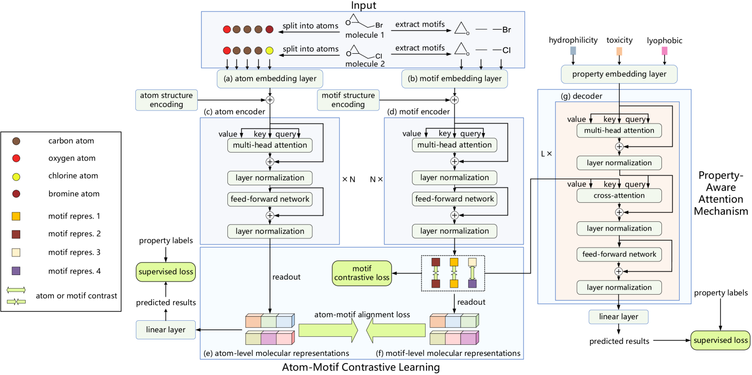
The Atom-Motif Contrastive Transformer (AMCT) framework can be viewed as a system designed to enhance the accuracy of market trend and pattern forecasting by integrating two levels of analysis: atomic elements and complex structures. The core idea is that candlesticks and the patterns formed from them are different representations of the same market scenario. This allows for a natural alignment of the two representations during the model training process. By extracting additional information inherent to these different levels of representation, the quality of the generated forecasts can be significantly improved.

Furthermore, similar market patterns observed across various timeframes or instruments typically produce similar signals. Therefore, the application of contrastive learning methods enables the identification of key patterns and enhances the quality of their interpretation. To more accurately identify patterns that play a critical role in determining market trends, the developers of the AMCT framework have introduced a property-aware attention mechanism that incorporates cross-attention techniques.

The original visualization of the Atom-Motif Contrastive Transformer framework as presented by the authors is provided below.

In the previous article, we discussed the implementation of candlestick and pattern pipelines, and we also constructed a relative cross-attention class, which we plan to use in the module analyzing the interdependencies between market scenario properties and candlestick patterns. Today, we will continue this work.

1. Analyzing Interdependencies Between Properties and Motifs

Let's take a closer look at the module responsible for analyzing interdependencies between properties and motifs. One of the key questions here is: what exactly do we mean by "properties"? At first glance, this might seem like a straightforward question, but in practice, it proves to be quite complex. The authors of the AMCT framework originally used various chemical properties they aimed to detect and analyze within molecular structures. But how can we define "properties" in the context of market scenarios — and more importantly, how can we describe them accurately?

Take the concept of a trend, for example. In classical technical analysis literature, trends are typically categorized into three types: uptrend, downtrend, and sideways. But the question arises — is this classification sufficient for in-depth analysis? How can we precisely describe the dynamics of price movement and the strength of a trend?

Even more questions emerge when selecting properties that characterize a market situation in the context of solving specific practical tasks.

If we don't yet have a clear solution to this problem, let's approach it from a different angle. Instead of manually defining market properties, we can allow the model to autonomously learn them from the training dataset — identifying features relevant to the task at hand. Much like the linguistic primitives learned in the RefMask3D framework, we will generate a learnable tensor of properties tailored to solving a specific applied problem. This is the algorithm we implement in the CNeuronPropertyAwareAttention class, the structure of which is presented below.

class CNeuronPropertyAwareAttention    :  public CNeuronRMAT
  {
protected:
   CBufferFloat      cTemp;
//---
   virtual bool      feedForward(CNeuronBaseOCL *NeuronOCL) override;
   virtual bool      calcInputGradients(CNeuronBaseOCL *NeuronOCL) override;
   virtual bool      updateInputWeights(CNeuronBaseOCL *NeuronOCL) override;

public:
                     CNeuronPropertyAwareAttention(void) {};
                    ~CNeuronPropertyAwareAttention(void) {};

   virtual bool      Init(uint numOutputs, uint myIndex, COpenCLMy *open_cl,
                          uint window, uint window_key, uint properties,
                          uint units_count, uint heads, uint layers,
                          ENUM_OPTIMIZATION optimization_type, uint batch);
   //---
   virtual int       Type(void) override   const   {  return defNeuronPropertyAwareAttention; }
  };

We use CNeuronRMAT as the parent class, which implements a linear model algorithm. As you may know, the internal components of our parent class are encapsulated within a single dynamic array. This design allows us to modify the internal architecture without declaring new member objects in the class structure. All that's required is to override the virtual object initialization method, where the necessary sequence of internal components is created. The only constraint is that the architecture must remain linear.

Unfortunately, the cross-attention architecture does not fully comply with the linearity requirement, as it operates with two separate input sources. As a result, we need to override the virtual methods for both the feed-forward and backpropagation passes. Let's take a closer look at the algorithms implemented in these overridden methods.

In the Init method, which initializes a new object, we receive constants that uniquely define the architecture of the object being created.

bool CNeuronPropertyAwareAttention::Init(uint numOutputs, uint myIndex, COpenCLMy *open_cl,
                                         uint window, uint window_key, uint properties,
                                         uint units_count, uint heads, uint layers,
                                         ENUM_OPTIMIZATION optimization_type, uint batch)
  {
   if(!CNeuronBaseOCL::Init(numOutputs, myIndex, open_cl, window * properties, optimization_type, batch))
      return false;

In the body of the method, we immediately call the relevant method from the base class of the fully connected neural layer - CNeuronBaseOCL.

It is important to note that in this case, we call the method from the base neural layer, not from the direct parent class. This is because our goal is to initialize only the base interfaces. The sequence of internal components will be completely redefined in our implementation.

Next, we prepare a dynamic array to store pointers to the internal components.

cLayers.Clear();
cLayers.SetOpenCL(OpenCL);

We also declare local variables to temporarily store the pointers to the objects we'll be creating.

CNeuronBaseOCL *neuron=NULL;
CNeuronRelativeSelfAttention *self_attention = NULL;
CNeuronRelativeCrossAttention *cross_attention = NULL;
CResidualConv *ff = NULL;

With this we complete the preparatory work and move on to constructing the sequence of internal objects. First, we create 2 consecutive fully connected layers to generate a trainable embedding tensor of features that can characterize the market situation.

int idx = 0;
neuron = new CNeuronBaseOCL();
if (!neuron ||
    !neuron.Init(window * properties, idx, OpenCL, 1, optimization, iBatch) ||
    !cLayers.Add(neuron))
    return false;
CBufferFloat *temp = neuron.getOutput();
if (!temp.Fill(1))
    return false;
idx++;
neuron = new CNeuronBaseOCL();
if (!neuron ||
    !neuron.Init(0, idx, OpenCL, window * properties, optimization, iBatch) ||
    !cLayers.Add(neuron))
    return false;

Here, we apply approaches that have been successfully validated in our previous work. The first layer contains a single neuron with a fixed value of 1. The second neural layer generates the required sequence of embeddings, which will be trained using the base functionality of the created object. Pointers to both objects are added to our dynamic array in the order in which they are called.

We then proceed to construct a structure that closely resembles a vanilla Transformer decoder. The only modification is that we replace the standard attention modules with equivalents that support relative positional encoding of the analyzed sequence structure. To achieve this, we create a loop with the number of iterations equal to the specified number of internal layers.

for (uint i = 0; i < layers; i++) 
  {
    idx++;
    self_attention = new CNeuronRelativeSelfAttention();
    
    if (!self_attention ||
        !self_attention.Init(0, idx, OpenCL, window, window_key, properties, heads, optimization, iBatch) ||
        !cLayers.Add(self_attention)
       ) 
       {
        delete self_attention;
        return false;
       }

Inside the loop body, we first create and initialize a relative Self-Attention layer that analyzes the interdependencies between the embeddings of the learnable properties characterizing the market situation in the context of the task being solved. Therefore, the length of the sequence being analyzed is determined by the properties parameter. A pointer to the newly created object is then added to our dynamic array.

Next, we create a relative cross-attention layer.

idx++;
cross_attention = new CNeuronRelativeCrossAttention();

if (!cross_attention ||
    !cross_attention.Init(0, idx, OpenCL, window, window_key, properties, heads, window, units_count,
                          optimization, iBatch) ||
    !cLayers.Add(cross_attention)
   ) 
   {
    delete cross_attention;
    return false;
  }

Here again, the embeddings of the properties serve as the primary input stream, which determines the shape of the result tensor. Consequently, the length of the sequence in the FeedForward block is also set equal to the number of generated properties.

idx++;
ff = new CResidualConv();
if (!ff ||
    !ff.Init(0, idx, OpenCL, window, window, properties, optimization, iBatch) ||
    !cLayers.Add(ff)
   ) 
   {
    delete ff;
    return false;



   }
}

We add pointers to these newly created objects to the dynamic array and proceed to the next iteration of the loop.

Once the required number of iterations is successfully completed, our dynamic array contains the full set of objects needed for the correct implementation of the module that analyzes interdependencies between the learnable properties and the detected patterns. The final step is to substitute the data buffer pointers, which allows us to significantly reduce the number of operations during model training.

if (!SetOutput(ff.getOutput()) ||
    !SetGradient(ff.getGradient()))
    return false;
//---
   return true;



  }

We conclude the method by returning a boolean result indicating the success of the operations to the calling program.

Once the initialization of the new object of our class is complete, we proceed to implement the feed forward-pass algorithm, defined in the feedForward method. It's important to note that even though our block architecture includes a cross-attention module, the feed-forward pass method receives only a single pointer to the input data object. This is because the second input source (the "properties") is generated internally by the objects of our class.

bool CNeuronPropertyAwareAttention::feedForward(CNeuronBaseOCL *NeuronOCL)
  {
   if(!NeuronOCL)
      return false;

In the body of the method, we immediately check the relevance of the received pointer. Since this object will be used as an additional data source, we will be accessing its data buffers directly. An invalid pointer at this stage could result in a critical failure.

We declare a local variable to temporarily store the pointer to the input object.

CNeuronBaseOCL *neuron = NULL;

Note that we declare this variable using the base type of our neural layers. This base type serves as a common ancestor for all our internal neural layer objects. This allows us to store a pointer to any of the internal components in the declared variable and use their base interfaces and overridden methods.

We then proceed to work with our property embedding generation model. Its objects are stored in the first two elements of our dynamic array. The first neural layer contains a fixed value, so we immediately call the feed-forward method of the second object, passing the pointer to the first layer as input.

if (bTrain) 
   {
    neuron = cLayers[1];
    if (!neuron || 
        !neuron.FeedForward(cLayers[0]))
        return false;
   }

However, we only call the feed-forward method of the second layer during training, because at this stage the model learns to extract property embeddings from the training data that are relevant to the current task. During the operational use, we instead use the previously learned property embeddings. As a result, the output of this layer remains constant. And there's no need to regenerate the embedding tensor on each pass. Skipping this step during real-world operation reduces the model's decision-making latency.

After that, we simply iterate through the remaining internal layers, sequentially calling their feedForward methods. As inputs, we provide the output of the previous layer along with the result buffer of the input object received in the method parameters.

for (int i = 2; i < cLayers.Total(); i++) 
  {
    neuron = cLayers[i];
    if (!neuron.FeedForward(cLayers[i - 1], NeuronOCL.getOutput()))
        return false;
  }
//---
   return true;
  }

The primary data source here is the output of the previous layer. This is the main data stream through which the embeddings of the learnable properties of market situations are passed. These embeddings are processed by all attention modules and the FeedForward block in the Decoder. The pattern embeddings, received as a parameter in the method, represent patterns detected in the description of the analyzed market situation. They highlight the properties most relevant to the current context. As a result, the Decoder outputs a refined representation of the market situation as a set of properties with emphasis on the most important features.

After completing all iterations of the loop, the feedForward method concludes by returning a boolean indicating the success of the operation to the calling function.

Next, we need to construct the backpropagation process. The updateInputWeights method, which updates model parameters, is quite simple. We simply call the corresponding method on each internal object in sequence. However, the calcInputGradients method, which distributes error gradients, includes a more nuanced detail.

As you know, the gradient distribution algorithm must exactly mirror the information flow of the feed-forward pass but in reverse order, distributing the error gradient among all components based on their contribution to the final output. If an object serves as a data source for multiple information flows, it must receive its share of the error gradient from each flow.

Take another look at the feed-forward pass implementation. The pattern embedding object pointer is passed as a parameter to all internal neural layers of the Decoder. Naturally, the Self-Attention and FeedForward modules will ignore it, since they don't use a second input source. However, the cross-attention modules will make use of these embeddings at each internal layer of the Decoder. Therefore, during error backpropagation, we must accumulate the corresponding portions of the error gradient from each cross-attention module and apply the sum to the pattern embedding object.

The method receives a pointer to the pattern embedding object as one of its parameters. The first step in the method body is to validate the pointer to ensure it is up to date and safe to use.

bool CNeuronPropertyAwareAttention::calcInputGradients(CNeuronBaseOCL *NeuronOCL)
  {
   if(!NeuronOCL)
      return false;

Next, we have some preparatory work to do. Here, we first check for the presence of a previously initialized auxiliary data buffer into which we plan to write intermediate values of the error gradients. We also need to make sure that its size is sufficient. In case of a negative result, at any control point we initialize a new data buffer of sufficient size.

if (cTemp.GetIndex() < 0 || cTemp.Total() < NeuronOCL.Neurons()) 
   {
    cTemp.BufferFree();
    if (!cTemp.BufferInit(NeuronOCL.Neurons(), 0) ||
        !cTemp.BufferCreate(OpenCL))
        return false;
   }

Then we reset the error gradient buffer obtained in the object parameters.

if (!NeuronOCL.getGradient() ||
    !NeuronOCL.getGradient().Fill(0))
    return false;

We usually do not perform this operation, since when performing error gradient distribution operations, we replace previously stored values with new ones. This is a good solution for linear models. But on the other hand, such an implementation forces us to look for workarounds in the case of collecting error gradients from several paths.

After successfully completing the preparatory work, we run a reverse loop through the internal layers of our block in order to distribute the error gradient across them.

CNeuronBaseOCL *neuron = NULL;
for (int i = cLayers.Total() - 2; i > 0; i--) 
  {
    neuron = cLayers[i];
    if (!neuron.calcHiddenGradients(cLayers[i + 1], NeuronOCL.getOutput(),
                                    GetPointer(cTemp),
                                    (ENUM_ACTIVATION)NeuronOCL.Activation()))
        return false;

In the body of the loop, we call the error gradient distribution method of each internal layer, passing the corresponding parameters to it. However, instead of providing the standard gradient buffer, we pass a pointer to our temporary data storage buffer. Once the method of the internal component executes successfully, we proceed to check the type of the neural layer. As we know, not all internal layers used a second data source. If the current layer is identified as a cross-attention module, we accumulate the error gradient associated with the second input source into the buffer of the pattern embedding object, summing it with the previously collected values.

if (neuron.Type() == defNeuronRelativeCrossAttention) {
    if (!SumAndNormilize(NeuronOCL.getGradient(), GetPointer(cTemp), NeuronOCL.getGradient(), 1, false, 0, 0, 0, 1))
        return false;
}
//---
return true;



}

After all iterations of the loop have been completed successfully, we return a bool result of the operation to the calling function and conclude the execution of the method.

With that, we complete the implementation of the property-aware attention block. The complete source code for this class and all its methods is provided in the attachment.

2. The AMCT Framework

We have made significant progress and implemented individual building blocks that constitute the Atom-Motif Contrastive Transformer (AMCT) framework. Now it is time to integrate these modules into a cohesive architecture. To do this, we will create an object called CNeuronAMCT. Its structure is shown below.

class CNeuronAMCT    :  public CNeuronBaseOCL
  {
protected:
   CNeuronRMAT                   cAtomEncoder;
   CNeuronMotifEncoder           cMotifEncoder;
   CLayer                        cMotifProjection;
   CNeuronPropertyAwareAttention cPropertyDecoder;
   CLayer                        cPropertyProjection;
   CNeuronBaseOCL                cConcatenate;
   CNeuronMHAttentionPooling     cPooling;
   //---
   virtual bool      feedForward(CNeuronBaseOCL *NeuronOCL) override;
   virtual bool      calcInputGradients(CNeuronBaseOCL *NeuronOCL) override;
   virtual bool      updateInputWeights(CNeuronBaseOCL *NeuronOCL) override;

public:
                     CNeuronAMCT(void) {};
                    ~CNeuronAMCT(void) {};
   //---
   virtual bool      Init(uint numOutputs, uint myIndex, COpenCLMy *open_cl,
                          uint window, uint window_key, uint properties,
                          uint units_count, uint heads, uint layers,
                          ENUM_OPTIMIZATION optimization_type, uint batch);
   //---
   virtual int       Type(void) override   const   {  return defNeuronAMCT; }
   //---
   virtual bool      Save(int const file_handle) override;
   virtual bool      Load(int const file_handle) override;
   //---
   virtual bool      WeightsUpdate(CNeuronBaseOCL *source, float tau) override;
   virtual void      SetOpenCL(COpenCLMy *obj) override;
  };

In the presented structure, we see the declaration of the objects we have implemented and two additional dynamic arrays. We will talk about their functionality a little later. All objects are declared as static, which allows us to leave the class constructor and destructor empty. Initialization of both inherited and newly declared members is performed in the Init method.

In the parameters of the initialization method, we receive the main constants that allow us to uniquely determine the architecture of the object being created.

bool CNeuronAMCT::Init(uint numOutputs, uint myIndex, COpenCLMy *open_cl,
                       uint window, uint window_key, uint properties,
                       uint units_count, uint heads, uint layers,
                       ENUM_OPTIMIZATION optimization_type, uint batch)
  {
   if(!CNeuronBaseOCL::Init(numOutputs, myIndex, open_cl, window * units_count, optimization_type, batch))
      return false;

In the method body, we immediately call the identically named method of the parent class, passing a portion of the received parameters to it.

You've probably noticed that the structure of this object does not include internal variables for storing the received parameter values. All constants that define the architecture of our class are used solely for the initialization of internal objects, and the necessary values will be stored in those objects. In both the feed-forward and backpropagation methods, we interact only with these internal components. Therefore, we avoid introducing unnecessary class-level variables.

Next, we move on to initializing the internal objects. We start by initializing two pipelines: one for candlesticks and the other for patterns.

int idx = 0;
if (!cAtomEncoder.Init(0, idx, OpenCL, window, window_key, units_count, heads, layers, optimization, iBatch))
    return false;
idx++;
if (!cMotifEncoder.Init(0, idx, OpenCL, window, window_key, units_count, heads, layers, optimization, iBatch))
    return false;

Despite the architectural differences between these pipelines, both will operate on the same input data source, and at this stage they receive identical initialization parameters.

From these two pipelines, we expect to obtain two representations of the analyzed market situation: at the candlestick level and at the pattern level. The AMCT framework proposes aligning these representations to enrich and refine their mutual understanding. However, it's important to note that the output tensor dimensions of the two pipelines differ. This fact significantly complicates the alignment process. To address this, we use a lightweight scaling model to transform the output of the pattern pipeline. Pointers to these scaling model objects are stored in a dynamic array named cMotifProjection.

We begin by initializing this dynamic array.

cMotifProjection.Clear();
cMotifProjection.SetOpenCL(OpenCL);

We determine the length of the sequence of patterns. As you know, at the output of the pattern pipeline we get a concatenated tensor of embeddings of two levels.

int motifs = int(cMotifEncoder.Neurons() / window);

Note that the representation tensors differ only in the length of their sequences. The vector size describing each sequence element remains the same. Therefore, it makes perfect sense that the scaling process will operate on individual univariate sequences within the tensor. To do this, we first transpose the pattern-level representation tensor.

idx++;
CNeuronTransposeOCL *transp = new CNeuronTransposeOCL();
if (!transp ||
    !transp.Init(0, idx, OpenCL, motifs, window, optimization, iBatch) ||
    !cMotifProjection.Add(transp))
    return false;

We then apply a convolutional layer to scale these univariate sequences.

idx++;
CNeuronConvOCL *conv = new CNeuronConvOCL();
if (!conv ||
    !conv.Init(0, idx, OpenCL, motifs, motifs, units_count, 1, window, optimization, iBatch) ||
    !cMotifProjection.Add(conv))
    return false;
conv.SetActivationFunction((ENUM_ACTIVATION)cAtomEncoder.Activation());

Pay attention that the input window size and its stride are both equal to the length of the sequence in the pattern-level representation. Meanwhile, the number of filters is set to match the sequence length of the candlestick-level representation.

Another important aspect is how we define the sequence length and the number of univariate sequences. In this case, we specify that the input sequence consists of a single element. The number of univariate sequences equals the vector size of a single sequence element from the input. This configuration allows us to assign individual learnable weight matrices for scaling each unitary sequence of the input data. In other words, each element of the original input sequence will be scaled using its own dedicated matrix. This enables a more flexible and fine-tuned transformation process.

It's also essential to synchronize the activation functions between the output of the convolutional scaling layer and the candlestick-level representation pipeline.

Once this is done, we transpose the scaled data back to its original layout using a data transposition layer.

idx++;
transp = new CNeuronTransposeOCL();
if (!transp ||
    !transp.Init(0, idx, OpenCL, window, units_count, optimization, iBatch) ||
    !cMotifProjection.Add(transp))
    return false;
transp.SetActivationFunction((ENUM_ACTIVATION)conv.Activation());

Next, we initialize the cross-attention block for properties and patterns, which is designed to output a property-level representation of the analyzed market state.

idx++;
if (!cPropertyDecoder.Init(0, idx, OpenCL, window, window_key, properties, motifs, heads, layers, optimization, iBatch))
    return false;

And now, we've arrived at the pivotal moment. At the output of the three major blocks, we obtain three distinct representations of a single market scenario under analysis. Moreover, each of these representations is structured as a tensor with different dimensions. So what’s next? How do we use them to solve practical problems? Which one should we choose to achieve the highest prediction quality?

I think we should use all three representations. We've already initialized the scaling model for the pattern representation. Now, we'll create an analogous model for scaling the property-based representation. Pointers to these scaling model objects will be stored in the cPropertyProjection dynamic array.

cPropertyProjection.Clear();
cPropertyProjection.SetOpenCL(OpenCL);
idx++;
transp = new CNeuronTransposeOCL();
if (!transp ||
    !transp.Init(0, idx, OpenCL, properties, window, optimization, iBatch) ||
    !cPropertyProjection.Add(transp))
    return false;
idx++;
conv = new CNeuronConvOCL();
if (!conv ||
    !conv.Init(0, idx, OpenCL, properties, properties, units_count, 1, window, optimization, iBatch) ||
    !cPropertyProjection.Add(conv))
    return false;
conv.SetActivationFunction((ENUM_ACTIVATION)cAtomEncoder.Activation());
idx++;
transp = new CNeuronTransposeOCL();
if (!transp ||
    !transp.Init(0, idx, OpenCL, window, units_count, optimization, iBatch) ||
    !cPropertyProjection.Add(transp))
    return false;
transp.SetActivationFunction((ENUM_ACTIVATION)conv.Activation());

The three representations, brought to a unified dimensionality, are concatenated into a single tensor.

idx++;
if (!cConcatenate.Init(0, idx, OpenCL, 3 * window * units_count, optimization, iBatch))
    return false;

We have obtained a concatenated tensor that combines three diverse perspectives on a single market situation. Doesn't this remind you of the results from multi-head attention? In fact, we essentially have the outputs of three heads, and to derive the final values, we utilize a dependency-based pooling layer.

idx++;
if(!cPooling.Init(0, idx, OpenCL, window, units_count, 3, optimization, iBatch))
   return false;

Next, we simply replace the data buffers in the inherited interfaces with the corresponding pooling objects. This allows us to avoid unnecessary data copying operations.

if (!SetOutput(cPooling.getOutput(), true) ||
    !SetGradient(cPooling.getGradient(), true))
    return false;
//---
return true;
}

We then conclude the initialization method, returning a boolean status to the calling program indicating success.

Having completed the initialization method of our object, we proceed to organize the feed-forward pass processes. As usual, the forward pass algorithm is implemented in the feedForward method.

bool CNeuronAMCT::feedForward(CNeuronBaseOCL *NeuronOCL)
  {
   if(!cAtomEncoder.FeedForward(NeuronOCL))
      return false;
   if(!cMotifEncoder.FeedForward(NeuronOCL))
      return false;

Among the method parameters, we receive a pointer to the raw input data object, which we immediately pass to our two representation pipelines: the candlestick-level and pattern-level.

The output from the pattern pipeline is forwarded to the cross-attention module working with properties and patterns.

if(!cPropertyDecoder.FeedForward(cMotifEncoder.AsObject()))
   return false;

At this stage, we have three distinct representations of the analyzed market situation. We bring them to a unified data scale. For this, we first apply scaling to the pattern-level representation.

//--- Motifs projection
   CNeuronBaseOCL *prev = cMotifEncoder.AsObject();
   CNeuronBaseOCL *current = NULL;
   for(int i = 0; i < cMotifProjection.Total(); i++)
     {
      current = cMotifProjection[i];
      if(!current ||
         !current.FeedForward(prev, NULL))
         return false;
      prev = current;
     }

We then perform an analogous scaling procedure on the property-level representation.

//--- Property projection
   prev = cPropertyDecoder.AsObject();
   for(int i = 0; i < cPropertyProjection.Total(); i++)
     {
      current = cPropertyProjection[i];
      if(!current ||
         !current.FeedForward(prev, NULL))
         return false;
      prev = current;
     }

Now, we can merge the three representations into a single tensor.

//--- Concatenate
   uint window = cAtomEncoder.GetWindow();
   uint units = cAtomEncoder.GetUnits();
   prev = cMotifProjection[cMotifProjection.Total() - 1];
   if(!Concat(cAtomEncoder.getOutput(), prev.getOutput(), current.getOutput(), cConcatenate.getOutput(),
                                                                         window, window, window, units))
      return false;

We use a pooling layer to compute a weighted aggregation of the results from these three representations.

//--- Out
   if(!cPooling.FeedForward(cConcatenate.AsObject()))
      return false;
//---
   return true;
  }

Thanks to the buffer pointer replacements made during initialization, we avoid copying data into the class interface buffers We simply complete the method, returning a boolean success flag to the caller.

The next step is to develop the backpropagation methods. Of particular interest algorithmically is the gradient distribution method calcInputGradients. The branched dependency structure between information flows, as proposed by the AMCT framework authors, heavily influences this method algorithm. Let's examine its implementation in detail.

As usual, the method receives a pointer to the preceding layer's object, into which the error gradient must be propagated according to the contribution of the input data to the final result.

bool CNeuronAMCT::calcInputGradients(CNeuronBaseOCL *NeuronOCL)
  {
   if(!NeuronOCL)
      return false;

We immediately verify the pointer validity, since any further operations become meaningless if it is invalid.

Then, we sequentially distribute the error gradient across the internal objects. Notably, thanks to the buffer pointer replacements for interface buffers, there is no need to copy data from external interfaces to internal objects. Thus, we can immediately begin distributing the error gradient across internal objects. We start by calculating the error gradient at the concatenated tensor representing the three perspectives of the analyzed environment state.

if(!cConcatenate.calcHiddenGradients(cPooling.AsObject()))
   return false;

We then propagate the error gradient to the individual pipelines. The gradient for the candlestick-level representation is immediately forwarded to the Encoder. The other two are passed to their respective scaling models.

uint window = cAtomEncoder.GetWindow();
uint units = cAtomEncoder.GetUnits();
CNeuronBaseOCL *motifs = cMotifProjection[cMotifProjection.Total() - 1];
CNeuronBaseOCL *prop = cPropertyProjection[cPropertyProjection.Total() - 1];
if (!motifs || !prop ||
    !DeConcat(cAtomEncoder.getGradient(), motifs.getGradient(), prop.getGradient(), cConcatenate.getGradient(),
              window, window, window, units))
    return false;

Next, we adjust the error gradients of the individual representations according to their activation functions.

if (cAtomEncoder.Activation() != None) {
    if (!DeActivation(cAtomEncoder.getOutput(), cAtomEncoder.getGradient(), cAtomEncoder.getGradient(),
                      cAtomEncoder.Activation()))
        return false;
if (motifs.Activation() != None) {
    if (!DeActivation(motifs.getOutput(), motifs.getGradient(), motifs.getGradient(),
                      motifs.Activation()))
        return false;
if (prop.Activation() != None) {
    if (!DeActivation(prop.getOutput(), prop.getGradient(), prop.getGradient(),
                      prop.Activation()))
        return false;

We also add the error gradient resulting from the alignment between the candlestick and pattern representations.

if(!motifs.calcAlignmentGradient(cAtomEncoder.AsObject(), true))
   return false;

Following this, we distribute the error gradients through the scaling models, iterating backward through their neural layers.

for (int i = cMotifProjection.Total() - 2; i >= 0; i--) 
  {
    motifs = cMotifProjection[i];
    if (!motifs || 
        !motifs.calcHiddenGradients(cMotifProjection[i + 1]))
        return false;
  }

for (int i = cPropertyProjection.Total() - 2; i >= 0; i--) 
  {
    prop = cPropertyProjection[i];
    if (!prop || 
        !prop.calcHiddenGradients(cPropertyProjection[i + 1]))
        return false;
  }

The error gradient from the property scaling model is passed to the cross-attention module for properties and patterns, and subsequently to the pattern Encoder.

if (!cPropertyDecoder.calcHiddenGradients(cPropertyProjection[0]) ||
    !cMotifEncoder.calcHiddenGradients(cPropertyDecoder.AsObject()))
    return false;

It should be noted that the outputs of the pattern Encoder are also used in the pattern representation scaling model. Therefore, we must incorporate the error gradient from this secondary information flow. To do this, we first save the pointer to the error gradient buffer of the pattern Encoder in a local variable. Then we replace it with the "donor" buffer.

As the donor object, we chose the concatenation layer of the three representations. Its error gradient has already been distributed among the corresponding information streams. Since this layer has no learnable parameters, we can safely clear its buffer. Additionally, this layer has the largest buffer size among all internal objects in our block, making it the optimal donor candidate.

After the buffer replacement, we retrieve the error gradient from the scaling model. We also sum the gradients from both information streams, restore the original buffer pointers. And finally, we propagate the error gradient to the input data level.

CBufferFloat *temp = cMotifEncoder.getGradient();
if (!cMotifEncoder.SetGradient(cConcatenate.getGradient(), false) ||
    !cMotifEncoder.calcHiddenGradients(cMotifProjection[0]) ||
    !SumAndNormilize(temp, cMotifEncoder.getGradient(), temp, window, false, 0, 0, 0, 1) ||
    !cMotifEncoder.SetGradient(temp, false) ||
    !NeuronOCL.calcHiddenGradients(cMotifEncoder.AsObject()))
    return false;

A similar situation arises at the input data level: the error gradient received from the pattern Encoder must be augmented by the contribution coming through the candlestick Encoder pipeline. We repeat the pointer replacement trick for another buffer object accordingly.

temp = NeuronOCL.getGradient();
if (!NeuronOCL.SetGradient(cConcatenate.getGradient(), false) ||
    !NeuronOCL.calcHiddenGradients(cAtomEncoder.AsObject()) ||
    !SumAndNormilize(temp, NeuronOCL.getGradient(), temp, window, false, 0, 0, 0, 1) ||
    !NeuronOCL.SetGradient(temp, false))
    return false;
//---
return true;
}

Now that the error gradient has been fully distributed among all model components and input data, the method concludes by returning a boolean result to the caller.

I would like to highlight two key points in this implementation. First, during buffer pointer replacement, we always save the original buffer pointer beforehand. When calling the pointer replacement method, we explicitly set a false flag that prevents the deletion of the previously stored buffer object. This approach preserves the buffer and allows its pointer to be restored later. If we used true as in the initialization method, we would have deleted the existing buffer object, causing critical errors upon future access.

Second, regarding the method architecture: the presented algorithm does not implement the contrastive representation learning for patterns as proposed by the AMCT authors. Recall, however, that we integrated representation diversification within the relative cross-attention object. Thus, effectively, we relocated the contrastive learning error injection point.

This concludes our review of the algorithmic construction of the Atom-Motif Contrastive Transformer framework. The full source code for all presented classes and methods is available in the attachment. There, you’ll also find the complete code for the environment interaction and model training programs. All of them have been copied over unchanged from previous works. Included are also environment interaction programs and training scripts. Here we have replaced one layer.

//--- layer 2
   if(!(descr = new CLayerDescription()))
      return false;
   descr.type = defNeuronAMCT;
   descr.window = BarDescr;                           // Window (Indicators to bar)
     {
      int temp[] = {HistoryBars, 100};                // Bars, Properties
      if(ArrayCopy(descr.units, temp) < (int)temp.Size())
         return false;
     }
   descr.window_out = EmbeddingSize / 2;              // Key Dimension
   descr.layers = 5;                                  // Layers
   descr.step = 4;                                    // Heads
   descr.batch = 1e4;
   descr.activation = None;
   descr.optimization = ADAM;
   if(!encoder.Add(descr))
     {
      delete descr;
      return false;
     }

A complete architectural description of the trainable models is provided in the attachment.

3. Testing

We have completed substantial work implementing the Atom-Motif Contrastive Transformer framework in MQL5, and it is time to evaluate the effectiveness of our approaches in practice. To this end, we train the model using new objects on real historical data, followed by validation of the trained policy in the MetaTrader 5 Strategy Tester over a time period outside the training set.

As usual, model training is performed offline on a pre-collected training dataset covering the entire 2023 year. Training is iterative, and after several iterations, the training dataset is updated. This provides the most accurate evaluation of the Agent's actions according to the current policy.

During training, we obtained a model capable of generating profits on both the training and test datasets. But there is one caveat. The resulting model executes very few trades. We even extended the testing period to three months. The test results are presented below.

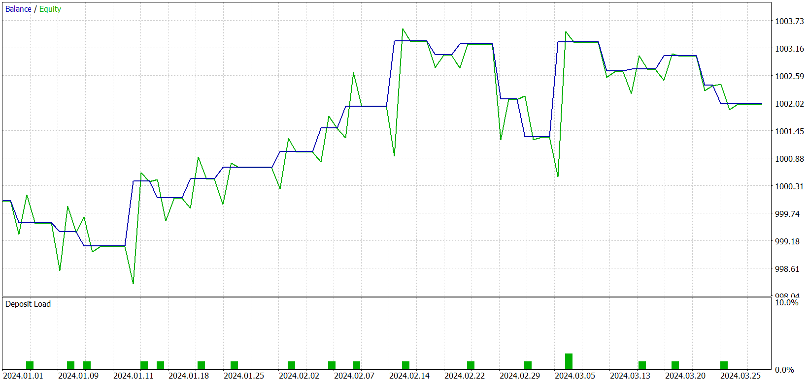
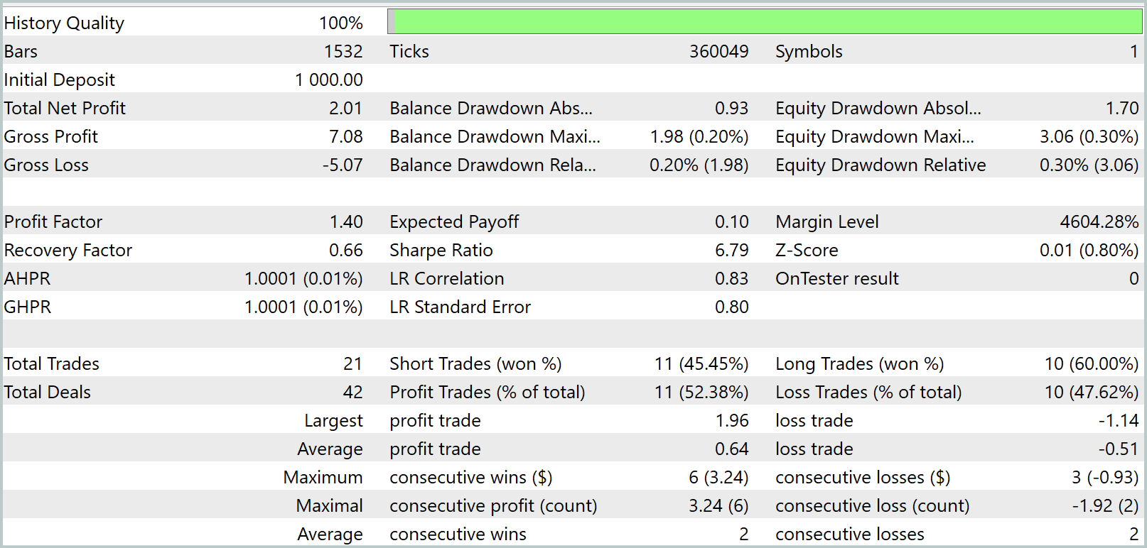
As can be seen from the results, over the three-month test interval, the model executed only 21 trades, with just over half closed profitably. Examining the balance graph, we observe an initial growth over the first month and a half, followed by sideways movement. This is quite expected behavior. Our model only collects statistics from market states present in the training dataset. Like any statistical model, the training set must be representative. From the balance graph, we can conclude that a one-year training dataset provides representativeness for approximately 1.2 to 1.5 months forward.

Thus, it can be hypothesized that training the model on a ten-year dataset may yield a model with stable performance over one year. Moreover, a larger training set should allow identification of a greater number of key patterns and learnable properties, potentially increasing trade frequency. However, confirming or refuting these hypotheses requires further work with the model.

Conclusion

In the last two articles, we have explored the Atom-Motif Contrastive Transformer (AMCT) framework, grounded in the concepts of atomic elements (candlesticks) and motifs (patterns). The main idea of the method is to apply contrastive learning to distinguish informative and non-informative patterns across multiple levels: from elemental components to complex structures. This enables the model not only to capture local price movements but also to detect significant patterns that provide additional insights for more accurate market behavior forecasting. The Transformer architecture underlying this framework effectively identifies long-term dependencies and intricate relationships between candlesticks and patterns.

In the practical part, we implemented our interpretation of these approaches in MQL5, trained the models, and conducted testing on real historical data. Unfortunately, the resulting model is sparse in trading activity. Nonetheless, there is evident potential, which we hope to further develop in future studies. 

References

• Atom-Motif Contrastive Transformer for Molecular Property Prediction
• Other articles from this series

Programs used in the article

#	Name	Type	Description
1	Research.mq5	Expert Advisor	EA for collecting examples
2	ResearchRealORL.mq5	Expert Advisor	EA for collecting examples using the Real-ORL method
3	Study.mq5	Expert Advisor	Model training EA
4	Test.mq5	Expert Advisor	Model testing EA
5	Trajectory.mqh	Class library	System state description structure
6	NeuroNet.mqh	Class library	A library of classes for creating a neural network
7	NeuroNet.cl	Library	OpenCL program code library