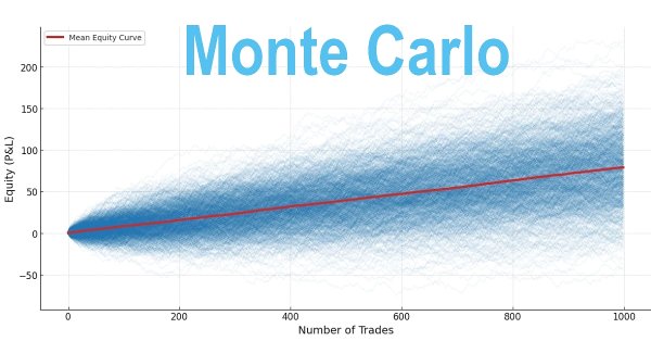
Building a Profitable Trading System (Part 1): A Quantitative Approach

Introduction

A consistently profitable trading system relies on the interplay of three core pillars:

1. Win Rate
2. Reward-to-Risk Ratio (RRR)
3. Risk Amount (via position sizing)

These three variables are fundamental drivers of key performance metrics such as profit factor, recovery factor, and drawdowns. However, many traders make the mistake of focusing almost exclusively on win rate, overlooking the critical importance of RRR and position sizing when evaluating the effectiveness of their (automated) trading systems.

To succeed eventually and remain active in the markets, traders must understand the dynamics of their trading edge—specifically its win rate, RRR, and the optimal position size that corresponds to those two metrics.

This article is designed to help traders evaluate their strategies over the long term by incorporating statistical results from back-testing into a Monte Carlo simulation. This approach generates a wide range of possible outcomes and provides an added layer of confidence—helping the trader determine whether a system should be continued, improved, or discarded.

Expectancy: The Math Behind Profitability

Profitability is quantified by expectancy—a function of win-rate and RRR. A positive expectancy defines a profitable system; A negative expectancy ensures long-term failure, no matter how impressive the win rate appears. However, even with positive expectancy, poor position sizing can amplify drawdowns beyond recovery.

What This Article Covers:

• The mathematical foundations of profitable trading systems
• Minimum thresholds required to achieve profitability
• Validation of strategy performance using Monte Carlo simulation in Python

The goal is to give traders a framework for assessing whether a system is statistically viable. For instance, if a trader's win rate does not exceed the minimum required threshold for a given RRR, then long-term profitability cannot be expected—regardless of how promising the back-test may seem.

Monte Carlo simulation allows traders to model thousands of synthetic outcomes based on varying combinations of win rates, RRRs, and position sizes. This enables better strategy optimization even before live or historical back-testing begins.

For traders who already have back-tested results, the simulation can be used to input actual win rates, RRRs, and position size levels to forecast potential future performance over a number of trades. This statistical insight provides greater clarity and confidence in whether a system is worth relying on.

Definitions and mathematical Concepts

1. Win-rate

The win-rate is defined as the proportion of winning trades relative to total trade over a certain period, expressed as a percentage or the probability of winning trades over a given period. In this article, the win-rate is denoted by P. 

Example: if 40 wins in 100 trades, the win-rate is 40%.

2. Reward-to-Risk Ratio (RRR)

Ratio of reward (Take-profit) to risk (Stop-loss):

Example: If the take profit is 100 pips and the stop loss is 50 pips, then RRR = 2.

3. Position Sizing

Position sizing refers to how much capital is risked per trade. It can be calculated as:

Example: Risking $200 with a 50-pip stop-loss and $10/pip tick value,

the position size= 0.4 lots

4. Expectancy 

Expectancy denoted by Ev represents the expected return per trade and is calculated as

Ev >0 : Profitable system (Long term)

Ev <0 : Unprofitable system

Minimum Win-rate or RRR Threshold to achieve a profitable system

It is a mathematical fact that win-rate and RRR are interdependent. For any given win-rate, there is a minimum RRR required to achieve profitability. Likewise, when RRR is known, it requires a minimum win-rate to be profitable. A high win-rate alone does not validate an automated system’s performance unless accompanied by a well-defined risk-reward ratio (RRR).

A system with predefined stop loss and take profit settings has a fixed RRR. If the corresponding win-rate is below the minimum required, the system cannot sustain long-term profitability, even if it generates short-term gains that may mislead traders. This often results in eventual account blowouts.

Deriving the Profitability Condition

Let walk through the mathematical concept to understand it better

From the Expectancy formula: 

Ev =(win-rate*reward) - (1 - win-rate)*risk

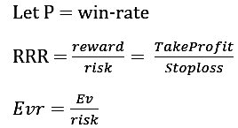
For a system to be profitable, Ev >0.

From equation 5:

If RRR is known, then the minimum win-rate(P) for a profitable system is given as:

If win-rate(P) is known, then the minimum RRR for a profitable system is given as:

Table 1: Minimum win-rate for a given RRR

RRR	minimum P
1.0	>50.00%
1.5	>40.00%
2.0	>33.33%
2.5	>28.57%
3.0	>25.00%

From Table 1, If a system has RRR=1, it needs more than 50%-win-rate to be profitable in a long term. Also, if a system has RRR=3.0, then it will require a win-rate of more than 25.00% to be profitable in a long term. It can be observed from the table 1 that as the RRR increases, the minimum win-rate decreases. If the RRR of a trading system exceeds its minimum win-rate, the system will be profitable in a long term.

Table 2: Minimum RRR required for a given win-rate

P	minimum RRR
30%	>2.333
40%	>1.50
50%	>1.00
60%	>0.667
70%	>0.429

Win-rate of a system is mostly not known unless back-test the strategy with historical data with a defined RRR. Table 2 gives us an idea of the minimum RRR for a particular win-rate to be profitable. With 30%-win-rate, RRR should be greater than 2.333 to achieve profitability in the long term. Likewise, with 70% win-rate, the RRR must exceed 0.429 to be profitable in the long term. As the win-rate increases, the RRR minimum decreases.

This is why traders should not blindly chase high win rates without considering RRR and vice versa.

Since the win-rate is simply the ratio of total winning trades to total trades, it’s important to allow the system to run long enough to gather sufficient trade data before drawing conclusions about its true win-rate. For example, an automated system that executes only 30 trades over 6 months and wins 20 of them would appear to have a 60% win-rate. However, if the same system—without any changes—is allowed to trade over18 months, executing 200 trades with 90 wins, the win-rate drops to 45%. The more trades the system completes, the more reliable and representative the win-rate becomes.

Position Sizing and Risk Management

The amount used to determine position sizing is typically expressed as a percentage of the account balance. This figure is critical because it determines whether a profitable trading system can endure periods of maximum drawdown, avoid blowing the account, and ultimately meet trading objectives.

Often, traders risk too large a percentage of their account in pursuit of quick profits, which can lead even a profitable system to wipe out their accounts. When this happens, the trader may blame the system developer, labeling the system a scam. The truth is: no matter how good or profitable a system is, as long as the win-rate isn’t 100%, it will experience losses. If you risk more than your account can handle, you will face margin calls and possibly a complete account wipe out if additional funds are unavailable to support it.

In this section, we’ll explore how to apply proper position sizing—staying within a safe risk zone—so you can survive losing streaks and still work toward your profit goals. This is the essence of sound risk or money management. Let’s dive into the math:

Definitions:

•  f: fixed fraction of the current account risked per trade.
•  RRRmin = 1.50: minimum reward-to-risk ratio
•  P = 0.40: Win-rate (40%)

Outcome of a winning Trade: 

if the trade wins, the gain is RRR * Amount risked

New Balance  = Current Balance + 1.50*(f*Current Balance)

Simplifying:

Outcome of a Losing Trade:

If the trade losses, the loss is the amount risked:

Expected Multiplicative Factor per Trade:

Combining Equation 8 & 9, the expected growth factor E[factor] is:

Substituting P=0.4 and simplifying gives:

Interpretation: At RRRmin = 1.50, the expected growth factor is exactly 1, meaning no long-term growth (breakeven).

Growth Condition

RRR> RRRmin :  For RRR =1.70

For positive growth (Ef >1); f must satisfy 

 

Calculating Optimal Risk fraction (f)

To achieve the target, say Ef = 1.002:

From this, we can see that we need to risk at least 2.5% of the account balance to reach our target. Risking less than 2.5% will allow the account to grow more steadily over time. This highlights an important concept that is often overlooked: for any given combination of win-rate, reward-to-risk ratio (RRR), and profit target, there is always a corresponding optimal risk per trade.

Expected Growth Factor 

To determine the Expected Growth Factor (Ef), a trader must first define three key parameters:

1. Profit target (P_target)
2. Number of trades to reach the target (x)
3. Initial account balance (Ini_bal)

Ef  is derived from a compound growth equation

For example, given the following:

• Profit target (P_target) = $10,000
• Number of trades (x) = 300
• Initial balance (Ini_bal) = $1,000

Plugging in the numbers gives:

The Expected Growth Factor reflects your trading style—whether you are a conservative or aggressive trader—because it determines the required risk per trade to achieve your target.

Example:

Suppose a trading system has:

Win-rate = 40%

Risk-reward ratio (RRR) = 1.7

A trader or automated system aims to grow $1000 into $10,000 over 300 trades. The required risk per trade (f) from equation 12 is calculated as:

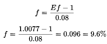
In this case, the trader or the automated system must risk at least 9.6% per trade to meet the target-an extreme aggressive approach.

Now if the number of trades to achieve the target is increased to x= 700:

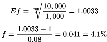
With 700 trades, the system or the trade becomes less aggressive, requiring only 4.1% risk per trade to reach the same target.

It is important to note that with a higher win-rate and had higher RRR, the target becomes more achievable.

Example:If RRR=2.0 (with P=40%), Ef = 1 + 0.2*f, reducing f to 1.54%  for Ef=1.0077

From this mathematical model, we can conclude that even profitable systems require optimizing both expectancy and position sizing. In the next section, we will illustrate this further using Monte Carlo simulations to provide a long-term perspective on the system’s potential.

Monte Carlo Simulation

To validate long-term robustness of a trading system depends on optimized RRR, win-rate and position sizing. Monte Carlo simulations will model the range of possible outcomes across thousands of randomized trade sequence. Parameters to optimize for are:

1. win-rate
2. RRR 
3. position sizing  

This will account for:

• Streaks of losses
• Maximum drawdowns
• Expected return paths
• Probability of account survival

However, the goal is to check for the expected returns and probability of account survival under different scenarios. 

The Monte Carlo simulation is built using python programming.

import numpy as np
import matplotlib.pyplot as plt

# Parameters
win_rate = 0.40
reward_risk_ratio = 1.5  # 1.5:1
risk_per_trade = 1  # Risk $1 per trade (normalized)
num_trades = 1000  # Total number of trades to simulate
num_simulations = 1000  # Number of Monte Carlo simulations

# Monte Carlo simulation
equity_curves = []

We import mathematical functions, multidimensional arrays and matrices need for computation using NumPy library and assign it as np.

We also import graphical functions for plotting our simulated results using the pyplot module from Matplotlib and gives it the alias plt.

We then initialize our win-rate, reward-risk-ratio, risk per trade, number of trades per each simulation and number of iterations. The results are stored in equity curves. The number of iterations can be reduced or increased depending on the user preference.

for _ in range(num_simulations):
    equity = 0
    curve = [equity] # Start curve with initial equity (0)
    peak = equity # Track peak equity for drawdown calculation
   # max_drawdown = 0 # Track max drawdown for this simulation

    for _ in range(num_trades):
        if np.random.rand() < win_rate:
            pnl = risk_per_trade * reward_risk_ratio
        else:
            pnl = -risk_per_trade
        equity += pnl
        curve.append(equity)

    equity_curves.append(curve)

# Convert to numpy array for easier analysis
equity_curves = np.array(equity_curves)

The simulation runs 1,000 iterations (100 trades each), stores results in an equity curve, and converts it to a NumPy array for analysis.

# Plot results
plt.figure(figsize=(12, 6))
for i in range(min(num_simulations, 100)):
    # Adjust indexing if plotting against trade number (starts from 0)
    plt.plot(range(num_trades + 1), equity_curves[i], alpha=0.2, color='blue')

The results of each simulation are plotted and displayed in blue.

# Plot mean curve
mean_curve = equity_curves.mean(axis=0)
plt.plot(range(num_trades + 1), mean_curve, color='red', linewidth=2, label='Mean Equity Curve')

A red line marks the average of the simulated results.

plt.title(f'Monte Carlo Simulation: {num_simulations} Simulations, {num_trades} Trades Each\nWin Rate = {win_rate*100:.1f}%, 
R:R = {reward_risk_ratio}:1')
plt.xlabel('Number of Trades')
plt.ylabel('Equity (P&L)')
plt.legend()
plt.grid(True)
plt.tight_layout() 
plt.show()

This segment handles plot formatting: title, axis labels (x-label, y-label), and grid activation (grid=True).

# Summary statistics
# Final equity is now the last element of the curve, which has num_trades + 1 points
final_equity = equity_curves[:, -1]
mean_final_equity = final_equity.mean()
median_final_equity = np.median(final_equity)
std_final_equity = final_equity.std()
percent_profitable = np.mean(final_equity > 0) * 100

print('mean_final_equity:',mean_final_equity, '\nmedian_final_equity:', median_final_equity,
 '\nstd_final_equity:', std_final_equity,'\npercent_profitable:', percent_profitable,'%')

The final code section calculates and prints: average final equity, median final equity, standard deviation of final equity, and percentage of profitable trades.

Scenario A: Performance of a Trading Strategy with 40% Win-Rate and 1.5 RRR Over 1,000 Simulations

In this scenario, a trading strategy with a win-rate of 40% and a reward-to-risk ratio (RRR) of 1.5 was tested across 1,000 trades per simulation. A total of 1,000 separate simulations were conducted to assess the strategy’s performance and risk characteristics. The results, summarized in Figure 1, are as follows:

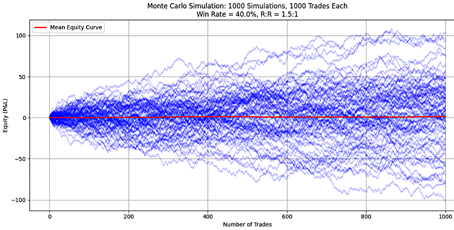
Figure 1

The simulation results for a 40% win rate and an RRR of 1.5 are as follows:

Stats	Values
Mean Final Equity	1.44
Median Final Equity	0.0
Standard Deviation of Final Equity	37.91
Percentage of Profitable Simulations	49.0%

Interpretation of Results

1. Mean Final Equity: The average final account balance across all simulations was 1.44 times the initial equity. This suggests that, on average, the strategy yielded a modest overall gain. However, this mean is significantly influenced by a few extreme positive outcomes, as illustrated in Figure 1. The presence of these outliers skews the mean upward, masking the frequency of poor results.

2. Median Final Equity: The median outcome was 0.0, indicating that at least half of the simulations resulted in a complete loss of capital. At least 50% of the simulations, the account was wiped out (likely hit 0 balance or margin called). The strategy has extreme risk of ruin. Half of the scenario lost the entire capital, while the other half generated profits, skewed enough to pull the mean up to 1.44. This shows most outcomes are poor and a red flag for unsustainable risk.

3. Standard Deviation: The standard deviation of 37.91 highlights the extreme volatility and unpredictability of the results. The standard deviation is large relative to the mean. Most paths cluster near total loss (mean=0). Some simulations ended up with large positive balance (which inflates the mean), while many crushed.

4. Percentage of Profitable Simulations: Only 49% of simulations ended profitably; thus, final equity ended above the initial balance. In 51% of runs, the system lost money. This aligns with the median=0.0 confirming that losses are catastrophic when they occur.

These statistical values reflect several key characteristics of the trading system's performance: 

• Unstable system:

Even though the mean final equity is positive(1.44x), the result is driven by a few “lucky” runs with high gains. The median being zero clearly shows that most runs performed terrible -at least 50% of them ended with an account blowout. This disparity between mean and median highlights a fundamentally unstable system—most runs perform very poorly, while only a few perform exceptionally well.

• High risk of ruin:

A median of zero demonstrated that this strategy has a high probability of blowing up your account unless very strict risk controls are applied.

• High volatility:

The large standard deviation (approximately 37.9) compared to the mean (approximately 1.44) suggests outcomes are extremely scattered. Some excellent, some disastrous. Such inconsistency makes it difficult to rely on this strategy for steady returns.

• Weak profitability:

Only 49% of the runs ended profitable, despite having a positive mean. The system does not prove to be reliable despite the positive mean because a stable, scalable system would have a much higher percentage of positive outcomes.

Scenario B: Performance of a Trading Strategy with 40% Win-Rate and 1.7 RRR Over 1,000 Simulations

In Scenario B, the trading strategy maintains a 40% win-rate but increased the reward-to-risk ratio (RRR) to 1.70 and was evaluated over 1,000 trades per simulation.  To thoroughly assess performance and risk characteristics, 1,000 separate Monte Carlo simulations were conducted. The key results, summarized in Figure 2, are as follows:

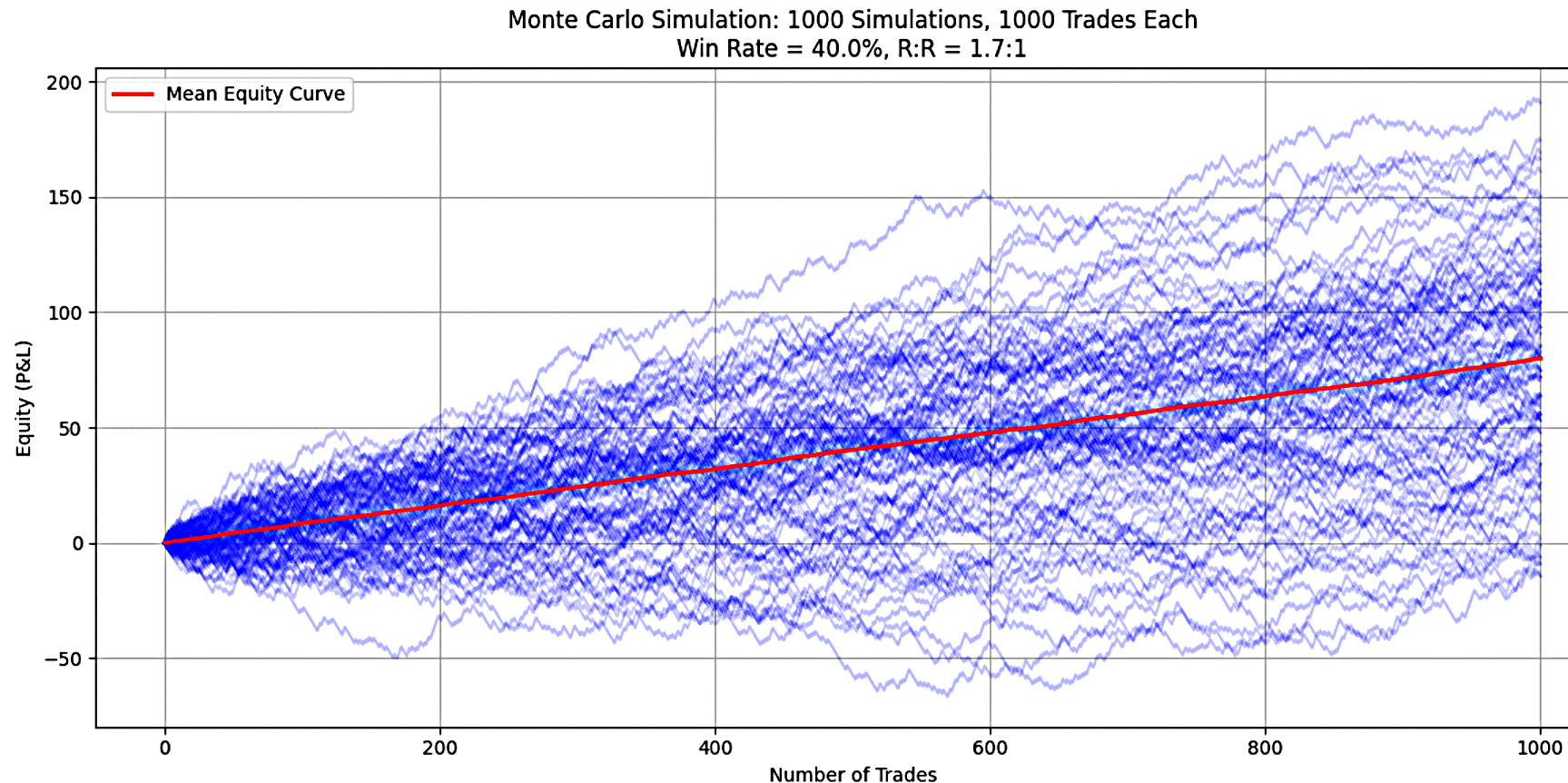
Figure 2

Below are the simulation outcomes for a 40% win rate with a 1.7 risk-reward ratio

Stats	Values
Mean Final Equity	80.0
Median Final Equity	80.0
Standard Deviation of Final Equity	45.82
Percentage of Profitable Simulations	96.7%

Interpretation of Results

1. Mean Final Equity: On average, the strategy grew the initial capital by 80 times over the simulation period. This reflects extraordinary compounding potential and confirms the strategy's strong profitability under these conditions. An average returns of 80x the initial balance is an outstanding result, suggesting that the system is capable of delivering substantial gains.

2. Median Final Equity:The median outcome was also 80x the initial capital, meaning that at least 50% of the simulations achieved returns at or above this level. The close alignment between the mean and median indicates a symmetrical distribution of outcomes, with most simulations clustered around the 80x return mark. This result highlights not only strong profitability but also excellent consistency across simulation runs. 

3. Standard Deviation of Final Equity: While the standard deviation of 45.82 indicates some variability in outcomes, this level of volatility is relatively modest when considered in relation to the considerable mean. The standard deviation is approximately 57% of the mean, suggesting that while individual results may vary (with some runs producing, for example, 40x or 120x returns), the majority of the outcomes remain concentrated around the 80x average. This reflects a system with controlled volatility and dependable performance.

4. Percentage of Profitable Simulations:An impressive 96.7% of simulations ended profitably, with only 3.3% resulting in a loss. This very high success rate demonstrates a system with exceptional reliability and a very low risk of ruin. The vast majority of trading runs produced gains, underscoring the robustness of the strategy under these simulated conditions.

These statistical values reflect several key characteristics of the trading system's performance: 

• Highly profitable:

The alignment of both the mean and median at 80x, combined with the tight clustering of results, demonstrates that this is a highly profitable and consistent system under the tested parameters.

• Low risk of ruin:

With only 3.3% of the simulations failing to turn a profit, the system shows a dramatic improvement in reliability over the earlier scenario with RRR of 1.5. The risk of ruin is now exceptionally low.

• Controlled volatility:

Although the absolute standard deviation appears large, it is reasonable compared to the very high returns. The outcomes suggest that while some variation is to be expected, the system consistently delivers strong results.

• Sensitivity to RRR:

The most striking observation is how, sufficiently, performance improved simply by increasing the RRR from 1.5 to 1.7 while keeping the win-rate at 40%. This underscores the importance of optimizing reward-to-risk ratios, particularly in strategies with lower win-rate, where even small adjustments can greatly enhance system stability and profitability.

Conclusion

This analysis has clearly demonstrated, both mathematically and through Monte Carlo simulations, that optimizing the reward-to-risk ratio (RRR) for a given win-rate can dramatically improve a trading system's profitability and stability. As shown in our scenarios, even maintaining a fixed win-rate of 40%, increasing the RRR from 1.5 to 1.7 transformed the system from one with high instability and significant risk of ruin to one delivering consistent profits with a low probability of account failure.

It is important to emphasize thatwin-rate and RRR are inherently interdependent, as shown in Equation 6 and 7 of this article. Effort to optimize RRR will naturally influence the effective win-rate and vice versa. Crucially, every win-rate has a corresponding minimum RRR that must be exceeded to achieve long-term profitability. For example, at a 40% win-rate, the system must surpass an RRR threshold of 1.5 to be sustainable.

This is further illustrated through expectancy:

At RRR=1.5 the Expectancy = (0.4*1.50)- (0.6*1) = 0. Suggesting breakeven. This explains the extreme divergence between the mean and the median.

At RRR=1.7, the Expectancy = (0.4*1.70)- (0.6*1) = 0.08. A positive expectancy, leading to a profitable outcome of 96.7%.

To conclude, many trading systems can be transformed into consistently profitable strategies by properly balancing win rate and RRR. The key is not merely achieving a high win rate, but ensuring that the RRR exceeds the minimum threshold required to generate positive expectancy over time.

When a trader defines both a stop loss and a take profit, the system’s RRR becomes fixed. For the system to be profitable during back-testing, the win rate must surpass the minimum required for that RRR. This article has provided several RRR values along with their corresponding minimum win rates. For other combinations, Equations 6 and 7 can be used to calculate the required profitability thresholds.

To evaluate long-term viability, traders can use Monte Carlo simulation to model performance based on their back-test statistics. By simulating thousands of possible trade sequences using your back-tested stats (win-rate, RRR, position sizing), Monte Carlo analysis:

• Projects the probability of success/failure over extended periods.
• Identifies whether results rely on luck or statistical edges.
• Empowers traders to trust their strategy—or revise it—before risking capital.

A system that consistently produces positive outcomes in simulation offers a higher degree of confidence, allowing traders to trust their strategy and maintain discipline.

Finally, while this article focused on expectancy and RRR optimization, it is important to emphasize that position sizing is an equally vital pillar of system performance. Without sound risk management, even a positive-expectancy system can fail. In the next article, we will explore how to apply optimal position sizing to improve system resilience and ensure sustainable trading success.