
Neural Networks in Trading: Optimizing the Transformer for Time Series Forecasting (LSEAttention)

Introduction
Multivariate time series forecasting plays a critical role across a wide range of domains (finance, healthcare, and more) where the objective is to predict future values based on historical data. This task becomes particularly challenging in long-term forecasting, which demands models capable of effectively capturing feature correlations and long-range dependencies in multivariate time series data. Recent research has increasingly focused on leveraging the Transformer architecture for time series forecasting due to its powerful Self-Attention mechanism, which excels at modeling complex temporal interactions. However, despite its potential, many contemporary methods for multivariate time series forecasting still rely heavily on linear models, raising concerns about the true effectiveness of Transformers in this context.
The Self-Attention mechanism at the core of the Transformer architecture is defined as follows:
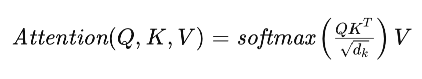
where Q, K, and V represent the Query, Key, and Value matrices respectively, and dk denotes the dimensionality of the vectors describing each sequence element. This formulation enables the Transformer to dynamically assess the relevance of different elements in the input sequence, thereby facilitating the modeling of complex dependencies within the data.
Various adaptations of the Transformer architecture have been proposed to improve its performance on long-term time series forecasting tasks. For example, FEDformer incorporates an advanced Fourier module that achieves linear complexity in both time and space, significantly enhancing scalability and efficiency for long input sequences.
PatchTST on the other hand, abandons pointwise attention in favor of patch-level representation, focusing on contiguous segments rather than individual time steps. This approach allows the model to capture more extensive semantic information in multivariate time series, which is crucial for effective long-term forecasting.
In domains such as computer vision and natural language processing, attention matrices can suffer from entropy collapse or rank collapse. This problem is further exacerbated in time series forecasting due to the frequent fluctuations inherent in time-based data, often resulting in substantial degradation of model performance. The underlying causes of entropy collapse remain poorly understood, highlighting the need for further investigation into its mechanisms and effects on model generalization. These challenges are the focus of the paper titled "LSEAttention is All You Need for Time Series Forecasting".
1. The LSEAttention Algorithm
The goal of multivariate time series forecasting is to estimate the most probable future values P for each of the C channels, represented as a tensor Y ∈ RC×P. This prediction is based on historical time series data of length L with C channels, encapsulated in the input matrix X ∈ RC×L. The task involves training a predictive model fωRC×L →RC×P parametrized by ω, to minimize the Mean Squared Error (MSE) between predicted and actual values.
Transformer rely heavily on pointwise Self-Attention mechanisms to capture temporal associations. However, this reliance can lead to a phenomenon known as attention collapse, where attention matrices converge to nearly identical values across different input sequences. This results in poor generalization of the data by the model.
The authors of the LSEAttention method draw an analogy between the dependency coefficients calculated via the Softmax function and the Log-Sum-Exp (LSE) operation. They hypothesize that numerical instability in this formulation may be the root cause of attention collapse.
The condition number of a function reflects its sensitivity to small input variations. A high condition number indicates that even minor perturbations in the input can cause significant output deviations.
In the context of attention mechanisms, such instability can manifest as over-attention or entropy collapse, characterized by attention matrices with extremely high diagonal values (indicating overflow) and very low off-diagonal values (indicating underflow).
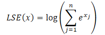
To address these issues, the authors propose the LSEAttention module, which integrates the Log-Sum-Exp (LSE) trick with the GELU (Gaussian Error Linear Unit) activation function. The LSE trick mitigates numerical instability caused by overflow and underflow through normalization. The Softmax function can be reformulated using LSE as follows:
![]()
where the exponent of LSE(x) denotes the exponential values of the log-sum-exp function, increasing numerical stability.
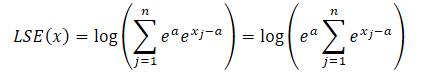
By using exponent properties, any exponential term can be expressed as the product of two exponential terms.
![]()
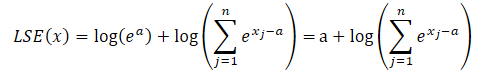
where a is a constant used for normalization. In practice, the maximum value is usually used as a constant. Substituting the product of the exponents into the LSE formula and taking the total value outside the sum sign, we have:
The logarithm of a product becomes a sum of logarithms, and the natural logarithm of an exponential equals the exponent. This allows us to simplify the expression presented:
Let's substituting the resulting expression into the Softmax function and use the exponential property:
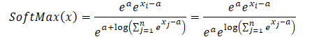
As you can notice, the exponential value of the constant common to the numerator and denominator is canceled out. The exponent of the natural logarithm is equal to the logarithmic expression. Thus, we obtain a numerically stable Softmax expression.
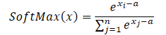
When using the maximum value as a constant (a = max(x)), we always get x-a less than or equal to 0. In this case, the exponential value from x-a lies in the range from 0 to 1, not including 0. Accordingly, the denominator of the function is in the range (1, n].
In addition, the authors of the LSEAttention framework propose using the GELU activation function, which provides smoother probabilistic activation. This helps stabilize extreme values in the logarithmic probability prior to applying the exponential function, thereby softening abrupt transitions in attention scores. By approximating the ReLU function through a smooth curve involving the cumulative distribution function (CDF) of the standard normal distribution, GELU reduces the sharp shifts in activations that can occur with traditional ReLU. This property is particularly beneficial for stabilizing Transformer-based attention mechanisms, where sudden activation spikes can lead to numerical instability and gradient explosions.
The GELU function is formally defined as follows:
![]()
where Φ(x) represents the CDF of the standard normal distribution. This formulation ensures that GELU applies varying degrees of scaling to input values depending on their magnitude, thereby suppressing the amplification of extreme values. The smooth, probabilistic nature of GELU enables a gradual transition of input activations, which in turn mitigates large gradient fluctuations during training.
This property becomes particularly valuable when combined with the Log-Sum-Exp (LSE) trick, which normalizes the Softmax function in a numerically stable manner. Together, LSE and GELU effectively prevent overflow and underflow in the exponential operations of Softmax, resulting in a stabilized range of attention weights. This synergy enhances the robustness of Transformer models by ensuring a well-distributed allocation of attention coefficients across tokens. Ultimately, this leads to more stable gradients and improved convergence during training.
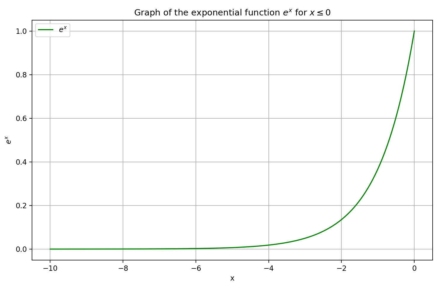
In traditional Transformer architectures, the ReLU (Rectified Linear Unit) activation function used in the Feed-Forward Network (FFN) block is prone to the "dying ReLU" problem, where neurons can become inactive by outputting zero for all negative input values. This results in zero gradients for those neurons, effectively halting their learning and contributing to training instability.
To address this issue, the Parametric ReLU (PReLU) function is used as an alternative. PReLU introduces a learnable slope for negative inputs, allowing non-zero output even when the input is negative. This adaptation not only mitigates the dying ReLU problem but also enables a smoother transition between negative and positive activations, thereby enhancing the model's capacity to learn across the entire input space. The presence of non-zero gradients for negative values supports better gradient flow, which is essential for training deeper architectures. Consequently, the use of PReLU contributes to overall training stability and helps maintain active representations, ultimately leading to improved model performance.
In the LSEAttention Time Series Transformer (LATST) architecture, the authors also incorporate invertible data normalization, which proves particularly effective in addressing distributional discrepancies between training and test data in time series forecasting tasks.
The architecture retains the traditional temporal Self-Attention mechanism, embedded within the LSEAttention module.
Overall, the LATST architecture consists of a single-layer Transformer structure augmented with substitution modules, enabling adaptive learning while maintaining the reliability of attention mechanisms. This design facilitates efficient modeling of temporal dependencies and boosts performance in time series forecasting tasks. The original visualization of the framework is provided below.
2. Implementation in MQL5
Having reviewed the theoretical aspects of the LSEAttention framework, we now turn to the practical part of our work, where we explore one possible implementation of the proposed techniques using MQL5. It's important to note that this implementation will differ significantly from previous ones. Specifically, we will not create a new object to implement the proposed methods. Instead, we will integrate them into previously developed classes.
2.1 Adjusting the Softmax layer
Let us consider the CNeuronSoftMaxOCL class, which handles the Softmax function layer. This class is extensively used both as a standalone component of our model and as part of various frameworks. For instance, we employed the CNeuronSoftMaxOCL object in building a pooling module based on dependency patterns (CNeuronMHAttentionPooling), which we have applied in several recent studies. Therefore, it is logical to incorporate numerically stable Softmax computations into this class algorithm.
To achieve this, we will modify the behavior of the SoftMax_FeedForward kernel. The kernel receives pointers to two data buffers as parameters: one for the input values and another for the output results.
__kernel void SoftMax_FeedForward(__global float *inputs,
                                  __global float *outputs)
  {
   const uint total = (uint)get_local_size(0);
   const uint l = (uint)get_local_id(0);
   const uint h = (uint)get_global_id(1);
We plan the execution of the kernel in a two-dimensional task space. The first dimension corresponds to the number of values to be normalized within a single unit sequence. The second dimension represents the number of such unit sequences (or normalization heads). We group threads into workgroups within each individual unit sequence.
Within the kernel body, we first identify the current thread in the task space across all dimensions.
We then declare a local memory array that will be used to facilitate data exchange within the workgroup.
__local float temp[LOCAL_ARRAY_SIZE];
Next, we define constant offsets into the global data buffers pointing to the relevant elements.
   const uint ls = min(total, (uint)LOCAL_ARRAY_SIZE);
   uint shift_head = h * total;
To minimize accesses to global memory, we copy the input values into local variables and validate the resulting values.
   float inp = inputs[shift_head + l];
   if(isnan(inp) || isinf(inp) || inp<-120.0f)
      inp = -120.0f;
It is worth noting that we limit the input values to a lower threshold of -120, which approximates the smallest exponent value representable in float format. This serves as an additional measure to prevent underflow. We do not impose an upper limit on values, as potential overflow will be addressed by subtracting the maximum value.
Next, we determine the maximum value within the current unit sequence. This is achieved through a loop that collects the maximums of each subgroup in the workgroup and stores them in elements of the local memory array.
   for(int i = 0; i < total; i += ls)
     {
      if(l >= i && l < (i + ls))
         temp[l] = (i > 0 ? fmax(inp, temp[l]) : inp);
      barrier(CLK_LOCAL_MEM_FENCE);
     }
We then iterate over the local array to identify the global maximum of the current workgroup.
   uint count = min(ls, (uint)total);
   do
     {
      count = (count + 1) / 2;
      if(l < ls)
         temp[l] = (l < count && (l + count) < total ? fmax(temp[l + count],temp[l]) : temp[l]);
      barrier(CLK_LOCAL_MEM_FENCE);
     }
   while(count > 1);
   float max_value = temp[0];
   barrier(CLK_LOCAL_MEM_FENCE);
The obtained maximum value is stored in a local variable, and we ensure thread synchronization at this stage. It is critical that all threads in the workgroup retain the correct maximum value before any modification of the local memory array elements occurs.
Now, we subtract the maximum value from each original input. Again, we check for the lower bound. Since subtracting a positive maximum may push the result beyond the valid range. We then compute the exponential of the adjusted value.
   inp = fmax(inp - max_value, -120);
   float inp_exp = exp(inp);
   if(isinf(inp_exp) || isnan(inp_exp))
      inp_exp = 0;
With two subsequent loops, we sum the resulting exponentials across the workgroup. The loop structure is similar to the one used to compute the maximum value. We just change the operation in the body of the loops accordingly.
   for(int i = 0; i < total; i += ls)
     {
      if(l >= i && l < (i + ls))
         temp[l] = (i > 0 ? temp[l] : 0) + inp_exp;
      barrier(CLK_LOCAL_MEM_FENCE);
     }
//---
   count = min(ls, (uint)total);
   do
     {
      count = (count + 1) / 2;
      if(l < ls)
         temp[l] += (l < count && (l + count) < total ? temp[l + count] : 0);
      if(l + count < ls)
         temp[l + count] = 0;
      barrier(CLK_LOCAL_MEM_FENCE);
     }
   while(count > 1);
Having obtained all required values, we can now compute the final Softmax values by dividing each exponential by the sum of exponentials within the workgroup.
//---
   float sum = temp[0];
   outputs[shift_head+l] = inp_exp / (sum + 1.2e-7f);
  }
The result of this operation is written to the appropriate element in the global result buffer.
It is important to highlight that the modifications made to the Softmax computation during the forward pass do not require changes to the backward pass algorithms. As shown in the mathematical derivations presented earlier in this article, the use of the LSE trick does not alter the final output of the Softmax function. Consequently, the influence of input data on the final result remains unchanged. Allowing us to continue using the existing gradient error distribution algorithm without modification.
2.2 Modifying the Relative Attention Module
It is important to note that the Softmax algorithm is not always used as a standalone layer. In nearly all versions of our implementations involving different Self-Attention block designs, its logic is embedded directly within a unified attention kernel. Let us examine the CNeuronRelativeSelfAttention module. Here, the entire algorithm for the modified Self-Attention mechanism is implemented within the MHRelativeAttentionOut kernel. And of course, we aim to ensure a stable training process across all model architectures. Therefore, we must implement numerically stable Softmax in all such kernels. Whenever possible, we retain the existing kernel parameters and task space configuration. This same approach was used in upgrading the MHRelativeAttentionOut kernel.
However, please note that any changes made to the kernel parameters or task space layout must be reflected in all wrapper methods of the main program that enqueue this kernel for execution. Failing to do so can result in critical runtime errors during kernel dispatch. This applies not only to modifications of the global task space but also to changes in workgroup sizes.
__kernel void MHRelativeAttentionOut(__global const float *q,         ///<[in] Matrix of Querys
                                     __global const float *k,         ///<[in] Matrix of Keys
                                     __global const float *v,         ///<[in] Matrix of Values
                                     __global const float *bk,        ///<[in] Matrix of Positional Bias Keys
                                     __global const float *bv,        ///<[in] Matrix of Positional Bias Values
                                     __global const float *gc,        ///<[in] Global content bias vector
                                     __global const float *gp,        ///<[in] Global positional bias vector
                                     __global float *score,           ///<[out] Matrix of Scores
                                     __global float *out,             ///<[out] Matrix of attention
                                     const int dimension              ///< Dimension of Key
                                    )
  {
//--- init
   const int q_id = get_global_id(0);
   const int k_id = get_local_id(1);
   const int h = get_global_id(2);
   const int qunits = get_global_size(0);
   const int kunits = get_local_size(1);
   const int heads = get_global_size(2);
Within the kernel body, as before, we identify the current thread within the task space and define all necessary dimensions.
Next, we declare a set of required constants, including both offsets into the global data buffers and auxiliary values.
   const int shift_q = dimension * (q_id * heads + h);
   const int shift_kv = dimension * (heads * k_id + h);
   const int shift_gc = dimension * h;
   const int shift_s = kunits * (q_id *  heads + h) + k_id;
   const int shift_pb = q_id * kunits + k_id;
   const uint ls = min((uint)get_local_size(1), (uint)LOCAL_ARRAY_SIZE);
   float koef = sqrt((float)dimension);
We also define a local memory array for inter-thread data exchange within each workgroup.
__local float temp[LOCAL_ARRAY_SIZE];
To compute attention scores according to the vanilla Self-Attention algorithm, we begin by performing a dot product between the corresponding vectors from the Query and Key tensors. However, the authors of the R-MAT framework add context-dependent and global bias terms. Since all vectors are of equal length, these operations can be carried out in a single loop, where the number of iterations equals the vector size. Within the loop body, we perform element-wise multiplication followed by summation.
//--- score
   float sc = 0;
   for(int d = 0; d < dimension; d++)
     {
      float val_q = q[shift_q + d];
      float val_k = k[shift_kv + d];
      float val_bk = bk[shift_kv + d];
      sc += val_q * val_k + val_q * val_bk + val_k * val_bk + gc[shift_q + d] * val_k + gp[shift_q + d] * val_bk;
     }
   sc = sc / koef;
The resulting score is scaled by the square root of the vector dimensionality. According to the authors of the vanilla Transformer, this operation improves model stability. We adhere to this practice.
The resulting values are then converted into probabilities using the Softmax function. Here, we insert operations to ensure numerical stability. First, we determine the maximum value among attention scores within each workgroup. To do this, we divide the threads into subgroups, each of which writes its local maximum to an element in the local memory array.
//--- max value
   for(int cur_k = 0; cur_k < kunits; cur_k += ls)
     {
      if(k_id >= cur_k && k_id < (cur_k + ls))
        {
         int shift_local = k_id % ls;
         temp[shift_local] = (cur_k == 0 ? sc : fmax(temp[shift_local], sc));
        }
      barrier(CLK_LOCAL_MEM_FENCE);
     }
We then loop over the array to find the global maximum value.
   uint count = min(ls, (uint)kunits);
//---
   do
     {
      count = (count + 1) / 2;
      if(k_id < ls)
         temp[k_id] = (k_id < count && (k_id + count) < kunits ?
                          fmax(temp[k_id + count], temp[k_id]) :
                                                    temp[k_id]);
      barrier(CLK_LOCAL_MEM_FENCE);
     }
   while(count > 1);
The current attention score is then adjusted by subtracting this maximum value before applying the exponential function. Here, we must also synchronize threads. Because in the next step, we will be changing the values of the local array elements and risk overwriting the value of the maximum element before it is used by all the threads of the workgroup.
   sc = exp(fmax(sc - temp[0], -120));
   if(isnan(sc) || isinf(sc))
      sc = 0;
   barrier(CLK_LOCAL_MEM_FENCE);
Next, we compute the sum of all exponentials within the workgroup. As before, we use a two-pass reduction algorithm consisting of sequential loops.
//--- sum of exp
   for(int cur_k = 0; cur_k < kunits; cur_k += ls)
     {
      if(k_id >= cur_k && k_id < (cur_k + ls))
        {
         int shift_local = k_id % ls;
         temp[shift_local] = (cur_k == 0 ? 0 : temp[shift_local]) + sc;
        }
      barrier(CLK_LOCAL_MEM_FENCE);
     }
//---
   count = min(ls, (uint)kunits);
   do
     {
      count = (count + 1) / 2;
      if(k_id < ls)
         temp[k_id] += (k_id < count && (k_id + count) < kunits ? temp[k_id + count] : 0);
      if(k_id + count < ls)
         temp[k_id + count] = 0;
      barrier(CLK_LOCAL_MEM_FENCE);
     }
   while(count > 1);
Now, we can convert the attention scores into probabilities by dividing each value by the total sum.
//--- score
   float sum = temp[0];
   if(isnan(sum) || isinf(sum) || sum <= 1.2e-7f)
      sum = 1;
   sc /= sum;
   score[shift_s] = sc;
   barrier(CLK_LOCAL_MEM_FENCE);
The resulting probabilities are written to the corresponding elements of the global output buffer, and we synchronize thread execution within the workgroup.
Finally, we compute the weighted sum of the Value tensor elements for each item in the input sequence. We will weigh the values based on the attention coefficients calculated above. Within one element of the sequence, this operation is represented by multiplying the vector of attention coefficients by the Value tensor, to which the authors of the R-MAT framework added global bias tensor.
This is implemented using a loop system, where the outer loop iterates over the last dimension of the Value tensor.
//--- out
   for(int d = 0; d < dimension; d++)
     {
      float val_v = v[shift_kv + d];
      float val_bv = bv[shift_kv + d];
      float val = sc * (val_v + val_bv);
      if(isnan(val) || isinf(val))
         val = 0;
Inside the loop, each thread computes its contribution to the corresponding element, and these contributions are aggregated using nested sequential reduction loops within the workgroup.
      //--- sum of value
      for(int cur_v = 0; cur_v < kunits; cur_v += ls)
        {
         if(k_id >= cur_v && k_id < (cur_v + ls))
           {
            int shift_local = k_id % ls;
            temp[shift_local] = (cur_v == 0 ? 0 : temp[shift_local]) + val;
           }
         barrier(CLK_LOCAL_MEM_FENCE);
        }
      //---
      count = min(ls, (uint)kunits);
      do
        {
         count = (count + 1) / 2;
         if(k_id < count && (k_id + count) < kunits)
            temp[k_id] += temp[k_id + count];
         if(k_id + count < ls)
            temp[k_id + count] = 0;
         barrier(CLK_LOCAL_MEM_FENCE);
        }
      while(count > 1);
The sum is then written to the appropriate element of the global result buffer by one of the threads.
      //---
      if(k_id == 0)
         out[shift_q + d] = (isnan(temp[0]) || isinf(temp[0]) ? 0 : temp[0]);
      barrier(CLK_LOCAL_MEM_FENCE);
     }
  }
Afterwards, we synchronize the threads again before moving on to the next loop iteration.
As discussed earlier, changes made to the Softmax function do not affect the dependence of results on the input data. Therefore, we are able to reuse the existing backpropagation algorithms without any modifications.
2.3 GELU Activation Function
In addition to numerical stabilization of the Softmax function, the authors of the LSEAttention framework also recommend using the GELU activation function. The authors proposed two versions of this function. One of them is presented below.
![]()
Implementing this activation function is quite simple. We just add the new variant to our existing activation function handler.
float Activation(const float value, const int function)
  {
   if(isnan(value) || isinf(value))
      return 0;
//---
   float result = value;
   switch(function)
     {
      case 0:
         result = tanh(clamp(value, -20.0f, 20.0f));
         break;
      case 1:  //Sigmoid
         result = 1 / (1 + exp(clamp(-value, -20.0f, 20.0f)));
         break;
      case 2:  //LReLU
         if(value < 0)
            result *= 0.01f;
         break;
      case 3:  //SoftPlus
         result = (value >= 20.0f ? 1.0f : (value <= -20.0f ? 0.0f : log(1 + exp(value))));
         break;
      case 4:  //GELU
         result = value / (1 + exp(clamp(-1.702f * value, -20.0f, 20.0f)));
         break;
      default:
         break;
     }
//---
   return result;
  }
However, behind the apparent simplicity of the feed-forward pass, there is a more complex task of implementing the backpropagation pass. This is because the derivative of GELU depends on the original input and the sigmoid function. Neither of them is available in our standard implementation.
![]()
Moreover, it is not possible to accurately express the derivative of the GELU function based solely on the result of the feed-forward pass. Therefore, we had to resort to certain heuristics and approximations.
Let\s begin by recalling the shape of the sigmoid function.
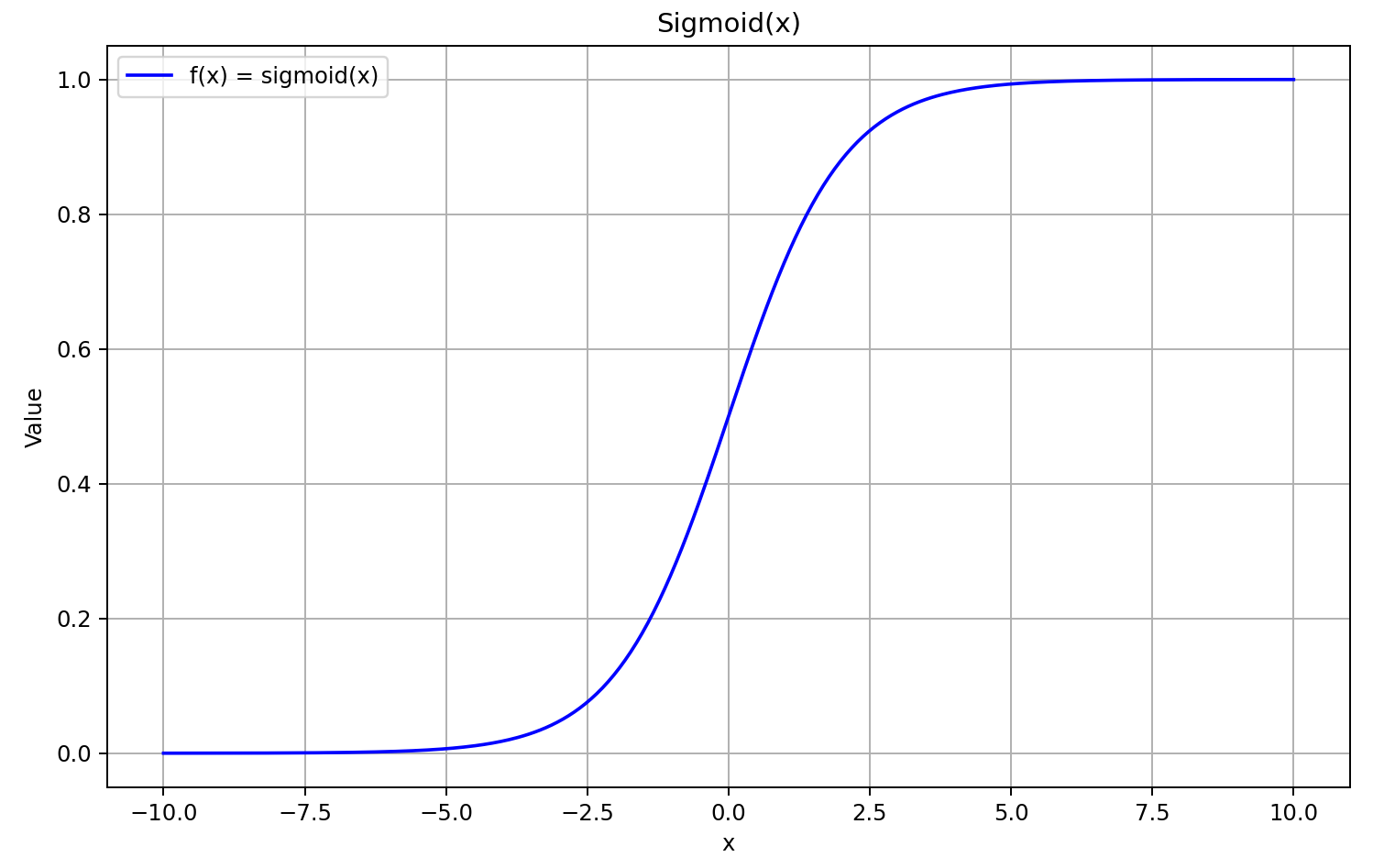
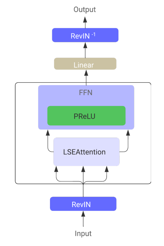
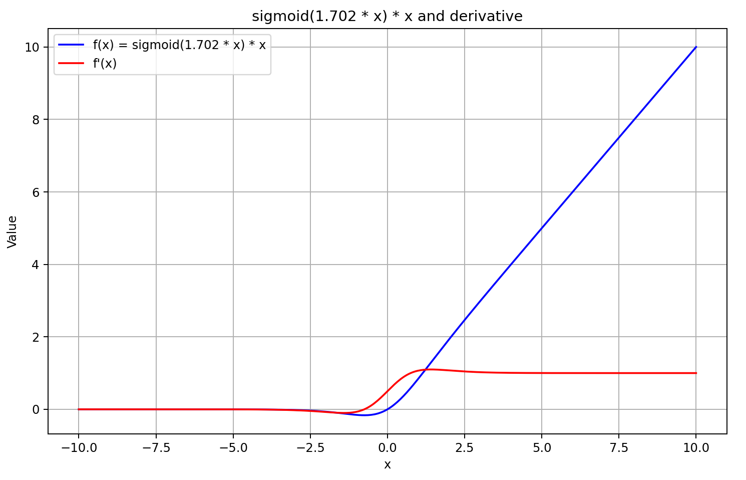
For input values greater than 5, the sigmoid approaches 1, and for inputs less than –5, it approaches 0. Therefore, for sufficiently negative values of X, the derivative of GELU tends toward 0, as the left-hand factor of the derivative equation approaches zero. For large positive values of X, the derivative tends toward 1, as both multiplicative factors converge to 1. This is confirmed by the graph shown below.
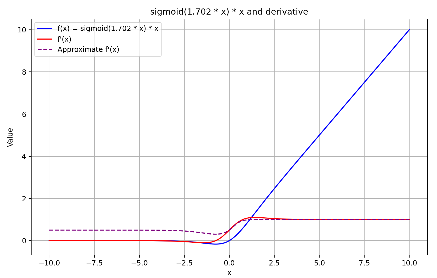
Guided by this understanding, we approximate the derivative as the sigmoid of the feed-forward pass result multiplied by 5. This method offers fast computation and produces a good approximation for GELU outputs greater than or equal to 0. However, for negative output values, the derivative is fixed at 0.5, due to which further training of the model cannot be continued. In reality, the derivative should approach 0, effectively blocking the propagation of the error gradient.
![]()
The decision has been made. Let's get started with implementation. To do this, we added another case to the derivative computation function.
float Deactivation(const float grad, const float inp_value, const int function)
  {
   float result = grad;
//---
   if(isnan(inp_value) || isinf(inp_value) ||
      isnan(grad) || isinf(grad))
      result = 0;
   else
      switch(function)
        {
         case 0: //TANH
            result = clamp(grad + inp_value, -1.0f, 1.0f) - inp_value;
            result *= 1.0f - pow(inp_value, 2.0f);
            break;
         case 1:  //Sigmoid
            result = clamp(grad + inp_value, 0.0f, 1.0f) - inp_value;
            result *= inp_value * (1.0f - inp_value);
            break;
         case 2: //LReLU
            if(inp_value < 0)
               result *= 0.01f;
            break;
         case 3:  //SoftPlus
            result *= Activation(inp_value, 1);
            break;
         case 4:  //GELU
            if(inp_value < 0.9f)
               result *= Activation(5 * inp_value, 1);
            break;
         default:
            break;
        }
//---
   return clamp(result, -MAX_GRAD, MAX_GRAD);
  }
Note that we compute the activation derivative only if the result of the feed-forward pass is less than 0.9. In all other cases, the derivative is assumed to be 1, which is accurate. This allows us to reduce the number of operations during gradient propagation.
The authors of the framework suggest using the GELU function as the non-linearity between layers in the FeedForward block. In our CNeuronRMAT class, this block is implemented using a feedback convolutional module CResidualConv. We modify the activation function used between layers within this module. This operation is done in the class initialization method. The specific update is underlined in the code.
bool CResidualConv::Init(uint numOutputs, uint myIndex, COpenCLMy *open_cl,
                         uint window, uint window_out, uint count,
                         ENUM_OPTIMIZATION optimization_type, uint batch)
  {
   if(!CNeuronBaseOCL::Init(numOutputs, myIndex, open_cl, window_out * count, optimization_type, batch))
      return false;
//---
   if(!cConvs[0].Init(0, 0, OpenCL, window, window, window_out, count, optimization, iBatch))
      return false;
   if(!cNorm[0].Init(0, 1, OpenCL, window_out * count, iBatch, optimization))
      return false;
   cNorm[0].SetActivationFunction(GELU);
   if(!cConvs[1].Init(0, 2, OpenCL, window_out, window_out, window_out, count, optimization, iBatch))
      return false;
   if(!cNorm[1].Init(0, 3, OpenCL, window_out * count, iBatch, optimization))
      return false;
   cNorm[1].SetActivationFunction(None);
//---

........
........
........
//---
   return true;
  }
With this, we complete the implementation of the techniques proposed by the authors of the LSEAttention framework. The full code of all modification can be found in the attachment, along with the full code for all programs used in preparing this article.
It should be noted that all environment interaction and model training programs were fully reused from the previous article. Similarly, the model architecture was left unchanged. This makes it all the more interesting to assess the impact of the introduced optimizations, since the only difference lies in the algorithmic improvements.
3. Testing
In this article, we implemented optimization techniques for the vanilla Transformer algorithm, as proposed by the authors of the LSEAttention framework, for time series forecasting. As previously stated, this work differs from our earlier studies. We did not create new neural layers, as done before. Instead, we integrated the proposed improvements into previously implemented components. In essence, we took the HypDiff framework implemented in the previous article and incorporated algorithmic optimizations that did not alter the model architecture. We also changed the activation function in the FeedForward block. These adjustments primarily affected the internal computation mechanisms by enhancing numerical stability. Naturally, we are interested in how these changes impact model training outcomes.
To ensure a fair comparison, we replicated the HypDiff model training algorithm in full. The same training dataset was used. However, this time we did not perform iterative updates to the training set. While this might slightly degrade training performance, it allows for an accurate comparison of the model before and after algorithm optimization.
The models were evaluated using real historical data from Q1 of 2024. The test results are presented below.
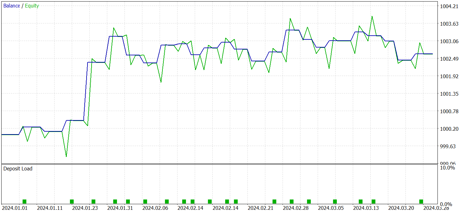
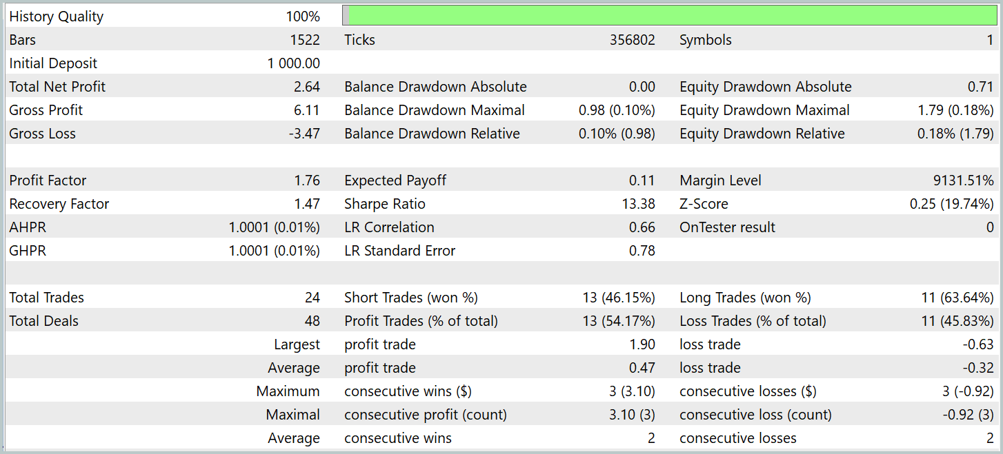
It should be noted that the model performance before and after modification was quite similar. During the test period, the updated model executed 24 trades. It deviated from the baseline model by only one trade, which falls within the margin of error. Both models made 13 profitable trades. The only visible improvement was the absence of a drawdown in February.
Conclusion
The LSEAttention method represents an evolution of attention mechanisms, particularly effective in tasks that demand high resilience to noise and data variability. The main advantage of LSEAttentionlies in the use of logarithmic smoothing, implemented via the Log-Sum-Exp function. This allows the model to avoid issues of numerical overflow and vanishing gradients, which are critical in deep neural networks.
In the practical section, we implemented the proposed approaches in MQL5, integrating them into previously developed modules. We trained and tested the models using real historical data. Based on the test results, we can conclude that these methods improve the stability of the model training process.
References
Programs used in the article
| # | Name | Type | Description |
|---|---|---|---|
| 1 | Research.mq5 | Expert Advisor | Expert Advisor for collecting examples |
| 2 | ResearchRealORL.mq5 | Expert Advisor | Expert Advisor for collecting examples using the Real-ORL method |
| 3 | Study.mq5 | Expert Advisor | Model training Expert Advisor |
| 4 | Test.mq5 | Expert Advisor | Model testing Expert Advisor |
| 5 | Trajectory.mqh | Class library | System state description structure |
| 6 | NeuroNet.mqh | Class library | A library of classes for creating a neural network |
| 7 | NeuroNet.cl | Library | OpenCL program code library |
Translated from Russian by MetaQuotes Ltd.
Original article: https://www.mql5.com/ru/articles/16360
Warning: All rights to these materials are reserved by MetaQuotes Ltd. Copying or reprinting of these materials in whole or in part is prohibited.
This article was written by a user of the site and reflects their personal views. MetaQuotes Ltd is not responsible for the accuracy of the information presented, nor for any consequences resulting from the use of the solutions, strategies or recommendations described.

 From Basic to Intermediate: Union (II)
- Free trading apps
- Over 8,000 signals for copying
- Economic news for exploring financial markets
You agree to website policy and terms of use