Neural Networks in Trading: Directional Diffusion Models (DDM)

Introduction
Unsupervised representation learning using diffusion models has become a key research area in computer vision. Experimental results from various researchers confirm the effectiveness of diffusion models in learning meaningful visual representations. The reconstruction of data distorted by varying levels of noise provides a suitable foundation for the model to grasp complex visual concepts. Moreover, prioritizing certain noise levels over others during training has been shown to improve the performance of diffusion models.
The authors of the paper "Directional Diffusion Models for Graph Representation Learning" proposed using diffusion models for unsupervised graph representation learning. However, they encountered limitations with "vanilla" diffusion models in practice. Their experiments revealed that data in graph structures often exhibits distinct anisotropic and directional patterns that are less pronounced in image data. Traditional diffusion models, which rely on an isotropic forward diffusion process, tend to suffer from a rapid decline in the internal signal-to-noise ratio (SNR), making them less effective for capturing anisotropic structures. To address this issue, the authors introduced novel approaches capable of efficiently capturing such directional structures. These include Directional Diffusion Models, which mitigate the problem of rapidly deteriorating SNR. The proposed framework incorporates data-dependent and directionally-biased noise into the forward diffusion process. Intermediate activations produced by the denoising model effectively capture valuable semantic and topological information that is critical for downstream tasks.
As a result, directional diffusion models offer a promising generative approach to graph representation learning. The authors' experimental results demonstrate that these models outperform both contrastive learning and traditional generative methods. Notably, for graph classification tasks, directional diffusion models even surpass baseline supervised learning models, highlighting the substantial potential of diffusion-based methods in graph representation learning.
Applying diffusion models within the context of trading opens up new possibilities for enhancing the representation and analysis of market data. Directional diffusion models, in particular, may prove especially useful due to their ability to account for anisotropic data structures. Financial markets are often characterized by asymmetric and directional movements, and models incorporating directional noise can more effectively recognize structural patterns in both trending and corrective phases. This capability enables the identification of hidden dependencies and seasonal trends.
1. The DDM Algorithm
There are significant structural differences between data found in graphs and in images. In the vanilla forward diffusion process, isotropic Gaussian noise is iteratively added to the original data until the data is completely transformed into white noise. This approach is appropriate when the data follows isotropic distributions, as it gradually degrades a data point into noise while generating noisy samples across a wide range of signal-to-noise ratios (SNR). However, for anisotropic data distributions, adding isotropic noise can quickly corrupt the underlying structure, causing a rapid drop in SNR to zero.
As a result, denoising models fail to learn meaningful and discriminative feature representations that can be effectively used for downstream tasks. In contrast, Directional Diffusion Models (DDMs), which incorporate a data-dependent and directional forward diffusion process, reduce the SNR at a slower rate. This more gradual degradation allows for the extraction of fine-grained feature representations across varying SNR levels, preserving crucial information about anisotropic structures. The extracted information can then be used for downstream tasks such as graph and node classification.
The generation of directional noise involves transforming the initial isotropic Gaussian noise into anisotropic noise through two additional constraints. These constraints are essential for improving the performance of diffusion models.
Let Gt = (A, Xt) represent the working state at the t-th step of the forward diffusion process, where 𝐗t = {xt,1, xt,2, …, xt,N} denotes the features being studied.
![]()
![]()
![]()
Here x0,i is the raw feature vector of node i, μ ∈ ℛ and σ ∈ ℛ represent the mean and standard deviation tensors of dimension d of features across all N nodes, respectively. And ⊙ denotes element-wise multiplication. During the mini-batch training, μ and σ are calculated using graphs within the batch. The parameter ɑt represents the fixed variance schedule and is parametrized by a decreasing sequence {β ∈ (0, 1)}.
Compared to the vanilla diffusion process, directional diffusion models impose two key constraints: One transforms the data-independent Gaussian noise into anisotropic, batch-specific noise. In this constraint, each coordinate of the noise vector is forced to match the empirical mean and standard deviation of the corresponding coordinate in the actual data. This limits the diffusion process to the local neighborhood of the batch, preventing excessive divergence and maintaining local coherence. Another constraint introduces as an angular direction that rotates the noise ε into the same hyperplane of the object x0,i, preserving its directional properties. This helps maintain the intrinsic structure of the data throughout the forward diffusion process.
These two constraints work in tandem to ensure that the forward diffusion process respects the underlying data structure and prevents rapid signal degradation. As a result, the signal-to-noise ratio decays more slowly, allowing directional diffusion models to extract meaningful feature representations across a range of SNR levels. This improves the performance of downstream tasks by providing more robust and informative embeddings.
The authors of the method follow the same training strategy used in vanilla diffusion models, training a denoising model fθ to approximate the reverse diffusion process. However, since the reverse of the forward process with directional noise cannot be expressed in closed form, the denoising model fθ is trained to directly predict the original sequence.
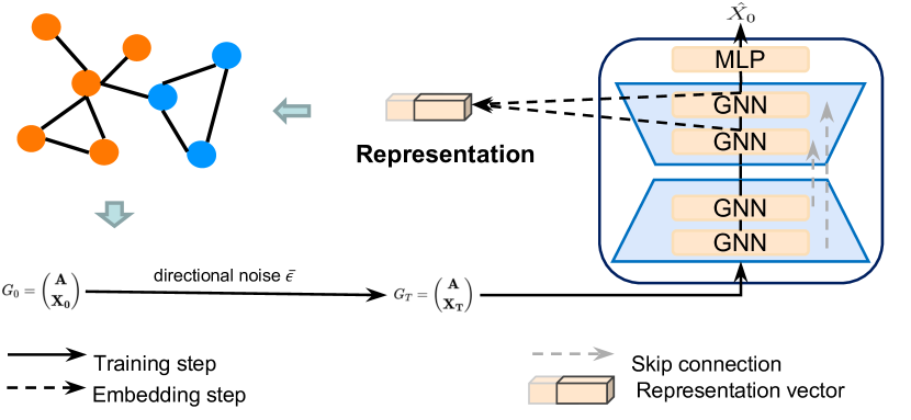
The original visualization of the Directional Diffusion Models framework as presented by the authors is provided below.
2. Implementation in MQL5
After considering the theoretical aspects of the Directional Diffusion Models method, we move on to the practical part of our article in which we implement the proposed approaches in MQL5.
We'll divide our work into two main sections. In the first stage, we will add directional noise to the data under analysis, and in the second stage, we will implement the framework within a single class structure.
2.1 Adding Directional Noise
And before we get started, let's discuss the algorithm of actions used for generating directional noise. First, we need noise from a normal distribution, which we can easily get using standard MQL5 libraries.
Next, following the methodology outlined by the authors of the framework, we must convert this isotropic noise into anisotropic, data-dependent noise. To do this, we need to compute the mean and variance for each feature. On closer inspection, this is similar to the task we already addressed when developing the batch normalization layer CNeuronBatchNormOCL. The batch normalization algorithm standardizes data to zero mean and unit variance. However, during the shift and scale phase, the data distribution is altered. In theory, we could extract this statistical information from the normalization layer itself. In fact, we previously implemented a procedure to obtain the parameters of the original distribution when developing the inverse normalization class CNeuronRevINDenormOCL. But this approach would constrain the flexibility and generality of our framework.
To overcome this limitation, we took a more integrated approach. We combined the addition of directional noise with the data normalization process itself. This raises an important question: At which point should the noise be added?
We can add noise BEFORE normalization. But this would distort the normalization process itself. Adding noise alters the data distribution. Therefore, applying normalization with previously computed mean and variance would result in a biased distribution. This would be an undesirable outcome.
The second option is to add noise at the output of the normalization layer. In this case, we would need to adjust the Gaussian noise by the scaling and shifting factors. But if you look at the above formulas of the original algorithm, you can see that this adjusting introduces bias, and the noise shifts towards the mean offset. Therefore, as the offset increases, we get skewed, asymmetric noise. Again, this is undesirable.
After weighing the pros and cons, we chose a different strategy: we add the noise between the normalization step and the scaling/offset application. This approach assumes the normalized data already has zero mean and unit variance. This is precisely the distribution we used to generate the noise. We then feed the noisy data into the scaling and shifting phase, allowing the model to learn appropriate parameters.
This will be the implementation strategy. We can proceed to the practical part of the work. The algorithm will be implemented on the OpenCL side. To that end, we will create a new kernel named BatchFeedForwardAddNoise. It's worth noting that the logic of this kernel is largely based on the feed-forward pass of the batch normalization layer. However, we extend it by adding a buffer for Gaussian noise data and a scaling factor for deviations, denoted as ɑ.
__kernel void BatchFeedForwardAddNoise(__global const float *inputs, __global float *options,
                                       __global const float *noise, __global float *output,
                                       const int batch, const int optimization,
                                       const int activation, const float alpha)
  {
   if(batch <= 1)
      return;
   int n = get_global_id(0);
   int shift = n * (optimization == 0 ? 7 : 9);
In the method body, we first check the size of the normalization batch, which must be greater than "1". Then we determine the offset into the data buffers based on the current thread ID.
Next, we check if the normalization parameter buffer contains real numbers. We will replace incorrect elements with zero values.
   for(int i = 0; i < (optimization == 0 ? 7 : 9); i++)
     {
      float opt = options[shift + i];
      if(isnan(opt) || isinf(opt))
         options[shift + i] = 0;
     }
We then normalize the original data in accordance with the base kernel algorithm.
   float inp = inputs[n];
   float mean = (batch > 1 ? (options[shift] * ((float)batch - 1.0f) + inp) / ((float)batch) : inp);
   float delt = inp - mean;
   float variance = options[shift + 1] * ((float)batch - 1.0f) + pow(delt, 2);
   if(batch > 0)
      variance /= (float)batch;
   float nx = (variance > 0 ? delt / sqrt(variance) : 0);
At this stage, we obtain normalized initial data with zero mean and unit variance. Here, we add noise, having previously adjusted its direction.
float noisex = sqrt(alpha) * nx + sqrt(1-alpha) * fabs(noise[n]) * sign(nx);
Then we perform the scaling and shifting algorithm, saving the results in the corresponding data buffers, similar to the implementation of the donor kernel. But this time, we apply scaling and offset to the noisy values.
   float gamma = options[shift + 3];
   if(gamma == 0 || isinf(gamma) || isnan(gamma))
     {
      options[shift + 3] = 1;
      gamma = 1;
     }
   float betta = options[shift + 4];
   if(isinf(betta) || isnan(betta))
     {
      options[shift + 4] = 0;
      betta = 0;
     }
//---
   options[shift] = mean;
   options[shift + 1] = variance;
   options[shift + 2] = nx;
   output[n] = Activation(gamma * noisex + betta, activation);
  }
We have implemented the feed-forward pass algorithm. What about the backpropagation pass? It should be noted here that to perform the backpropagation operations, we decided to use the full implementation of the batch normalization layer algorithms. The fact is that we do not train the noise itself. Therefore, the error gradient is passed directly and entirely to the original input data. The scaling factor ɑ we introduced earlier merely serves to blur the region around the original data slightly. Consequently, we can neglect this factor and forward the error gradients to the input in full accordance with the standard batch normalization algorithm.
Thus our work on the OpenCL side of the implementation is complete. The full source code is provided in the attachment. We now move to the MQL5 side of the implementation. Here, we will create a new class called CNeuronBatchNormWithNoise. As the name suggests, most of the core functionality is inherited directly from the batch normalization class. The only method that requires overriding is the feed-forward pass. The structure of the new class is shown below.
class CNeuronBatchNormWithNoise  :  public CNeuronBatchNormOCL
  {
protected:
   CBufferFloat      cNoise;
   //---
   virtual bool      feedForward(CNeuronBaseOCL *NeuronOCL);

public:
                     CNeuronBatchNormWithNoise(void) {};
                    ~CNeuronBatchNormWithNoise(void) {};
   //---
   virtual int       Type(void) const   {  return defNeuronBatchNormWithNoise;    }
  };
As you may have noticed, we tried to make the development of our new class CNeuronBatchNormWithNoise as straightforward as possible. Nevertheless, to enable the required functionality, we need a buffer to transfer the noise, which will be generated on the main side and passed into the OpenCL context. We deliberately chose not to override the object initialization method or file methods. There's no practical reason to keep randomly generated noise. Instead, all related operations are implemented within the feedForward method. This method receives a pointer to the input data object as a parameter.
bool CNeuronBatchNormWithNoise::feedForward(CNeuronBaseOCL *NeuronOCL)
  {
   if(!bTrain)
      return CNeuronBatchNormOCL::feedForward(NeuronOCL);
Pay attention that noise is added only during the training phase. This will help the model learn meaningful structures in the input data. During live usage, we want the model to act as a filter recovering meaningful patterns from real-world data that may inherently contain some level of noise or inconsistency. Therefore, no artificial noise is added at this stage. Instead, we perform standard normalization via the parent class functionality.
The following code is executed only during the model training process. We first check the relevance of the received pointer to the source data object.
if(!OpenCL || !NeuronOCL)
   return false;
And then we save it in an internal variable.
PrevLayer = NeuronOCL;
After that we check the size of the normalization package. And if it is not greater than 1, then we simply synchronize the activation functions and terminate the method with a positive result. Because in this case, the result of the normalization algorithm will be equal to the original data. To eliminate extra operations, we will simply pass the received initial data to the next layer.
if(iBatchSize <= 1)
  {
   activation = (ENUM_ACTIVATION)NeuronOCL.Activation();
   return true;
  }
If all the above checkpoints are successfully passed, we first generate noise from a normal distribution.
double random[];
if(!Math::MathRandomNormal(0, 1, Neurons(), random))
   return false;
After that we need to pass it to the OpenCL context. But we did not override the object initialization method. So we first check our data buffer to make sure it has enough elements and the previously created buffer is in context.
if(cNoise.Total() != Neurons() ||
   cNoise.GetOpenCL() != OpenCL)
  {
   cNoise.BufferFree();
   if(!cNoise.AssignArray(random))
      return false;
   if(!cNoise.BufferCreate(OpenCL))
      return false;
  }
When we get a negative value at one of the checkpoints, we change the buffer size and create a new pointer in the OpenCL context.
Otherwise, we simply copy the data into the buffer and move it into the OpenCL context memory.
else
  {
   if(!cNoise.AssignArray(random))
      return false;
   if(!cNoise.BufferWrite())
      return false;
  }
Next, we adjust the actual batch size and randomly determine the noise level of the original data.
iBatchCount = MathMin(iBatchCount, iBatchSize);
float noise_alpha = float(1.0 - MathRand() / 32767.0 * 0.01);
Now that we have prepared all the necessary data, we just need to pass it to the parameters of our kernel we've just created.
uint global_work_offset[1] = {0};
uint global_work_size[1];
global_work_size[0] = Neurons();
int kernel = def_k_BatchFeedForwardAddNoise;
ResetLastError();
if(!OpenCL.SetArgumentBuffer(kernel, def_k_normwithnoise_inputs, NeuronOCL.getOutputIndex()))
  {
   printf("Error of set parameter kernel %s: %d; line %d", OpenCL.GetKernelName(kernel),
                                                                    GetLastError(), __LINE__);
   return false;
  }
if(!OpenCL.SetArgumentBuffer(kernel, def_k_normwithnoise_noise, cNoise.GetIndex()))
  {
   printf("Error of set parameter kernel %s: %d; line %d", OpenCL.GetKernelName(kernel),
                                                                    GetLastError(), __LINE__);
   return false;
  }
if(!OpenCL.SetArgumentBuffer(kernel, def_k_normwithnoise_options, BatchOptions.GetIndex()))
  {
   printf("Error of set parameter kernel %s: %d; line %d", OpenCL.GetKernelName(kernel),
                                                                    GetLastError(), __LINE__);
   return false;
  }
if(!OpenCL.SetArgumentBuffer(kernel, def_k_normwithnoise_output, Output.GetIndex()))
  {
   printf("Error of set parameter kernel %s: %d; line %d", OpenCL.GetKernelName(kernel),
                                                                    GetLastError(), __LINE__);
   return false;
  }
if(!OpenCL.SetArgument(kernel, def_k_normwithnoise_activation, int(activation)))
  {
   printf("Error of set parameter kernel %s: %d; line %d", OpenCL.GetKernelName(kernel),
                                                                    GetLastError(), __LINE__);
   return false;
  }
if(!OpenCL.SetArgument(kernel, def_k_normwithnoise_alpha, noise_alpha))
  {
   printf("Error of set parameter kernel %s: %d; line %d", OpenCL.GetKernelName(kernel),
                                                                    GetLastError(), __LINE__);
   return false;
  }
if(!OpenCL.SetArgument(kernel, def_k_normwithnoise_batch, iBatchCount))
  {
   printf("Error of set parameter kernel %s: %d; line %d", OpenCL.GetKernelName(kernel),
                                                                    GetLastError(), __LINE__);
   return false;
  }
if(!OpenCL.SetArgument(kernel, def_k_normwithnoise_optimization, int(optimization)))
  {
   printf("Error of set parameter kernel %s: %d; line %d", OpenCL.GetKernelName(kernel),
                                                                    GetLastError(), __LINE__);
   return false;
  }
//---
if(!OpenCL.Execute(kernel, 1, global_work_offset, global_work_size))
  {
   printf("Error of execution kernel %s: %d; line %d", OpenCL.GetKernelName(kernel),
                                                                GetLastError(), __LINE__);
   return false;
  }
   iBatchCount++;
//---
   return true;
  }
And we put the kernel in the execution queue. We also control the operations at every step. At the end of the method, we return the logical result of the operations to the caller.
This concludes our new class CNeuronBatchNormWithNoise. Its full code is provided in the attached file.
2.2 The DDM Framework Class
We have implemented an object for adding directional noise to the original input data. And now we move on to building our interpretation of the Directional Diffusion Models framework.
We do use the structure of approaches proposed by the authors of the framework. However, we allow for some deviations in the context of our specific problems. In our implementation, we also use the U-shaped architecture proposed by the authors of the method, but replace Graph Neural Networks (GNN) to the Transformer encoder blocks. In addition, the authors of the method feed already noisy input into the model, while we add noise within the model itself. But first things first.
To implement our solution, we create a new class named CNeuronDiffusion. As a parent object, we use a U-shaped Transformer. The structure of the new class is shown below.
class CNeuronDiffusion  : public CNeuronUShapeAttention
  {
protected:
   CNeuronBatchNormWithNoise  cAddNoise;
   CNeuronBaseOCL             cResidual;
   CNeuronRevINDenormOCL      cRevIn;
   //---
   virtual bool      feedForward(CNeuronBaseOCL *NeuronOCL);
   virtual bool      calcInputGradients(CNeuronBaseOCL *prevLayer);
   virtual bool      updateInputWeights(CNeuronBaseOCL *NeuronOCL);

public:
                     CNeuronDiffusion(void) {};
                    ~CNeuronDiffusion(void) {};
   //---
   virtual bool      Init(uint numOutputs, uint myIndex, COpenCLMy *open_cl,
                          uint window, uint window_key, uint heads, uint units_count,
                          uint layers, uint inside_bloks,
                          ENUM_OPTIMIZATION optimization_type, uint batch);
   //---
   virtual int       Type(void)   const   {  return defNeuronDiffusion;   }
   //--- methods for working with files
   virtual bool      Save(int const file_handle);
   virtual bool      Load(int const file_handle);
   //---
   virtual bool      WeightsUpdate(CNeuronBaseOCL *source, float tau);
   virtual void      SetOpenCL(COpenCLMy *obj);
  };
In the presented class structure, we declared three new static objects, the purpose of which we will become familiar with during the implementation of the class methods. To build the basic architecture of the noise filtering model, we will use inherited objects.
All objects are declared as static, which allows us to leave the class constructor and destructor empty. The initialization of objects is performed in the Init method.
In the method parameters we receive the main constants that determine the architecture of the created object. It should be said that in this case, we have completely transferred the structure of the parameters from the parent class method without changes.
bool CNeuronDiffusion::Init(uint numOutputs, uint myIndex, COpenCLMy *open_cl,
                            uint window, uint window_key, uint heads,
                            uint units_count, uint layers, uint inside_bloks,
                            ENUM_OPTIMIZATION optimization_type, uint batch)
  {
   if(!CNeuronBaseOCL::Init(numOutputs, myIndex, open_cl, window * units_count, optimization_type, batch))
      return false;
However, while constructing new algorithms, we will slightly change the sequence in which the inherited objects will be used. Therefore, in the method body, we call the relevant method of the base class, in which only the main interfaces are initialized.
Next, we initialize the normalization object of the original input data with the addition of noise. We will use this object for the initial processing of the input data.
if(!cAddNoise.Init(0, 0, OpenCL, window * units_count, iBatch, optimization))
   return false;
We then build the U-shaped Transformer structure. Here, we first use the multi-headed attention block.
if(!cAttention[0].Init(0, 1, OpenCL, window, window_key, heads, units_count, layers, optimization, iBatch))
   return false;
This is followed by a convolutional layer for dimensionality reduction.
if(!cMergeSplit[0].Init(0, 2, OpenCL, 2 * window, 2 * window, window, (units_count + 1) / 2, optimization,
                                                                                                  iBatch))
   return false;
Then we recurrently form neck objects.
 if(inside_bloks > 0)
   {
    CNeuronDiffusion *temp = new CNeuronDiffusion();
    if(!temp)
       return false;
    if(!temp.Init(0, 3, OpenCL, window, window_key, heads, (units_count + 1) / 2, layers, inside_bloks - 1,
                                                                                     optimization, iBatch))
      {
       delete temp;
       return false;
      }
    cNeck = temp;
   }
 else
   {
   CNeuronConvOCL *temp = new CNeuronConvOCL();
   if(!temp)
      return false;
   if(!temp.Init(0, 3, OpenCL, window, window, window, (units_count + 1) / 2, optimization, iBatch))
     {
      delete temp;
         return false;
     }
   cNeck = temp;
     }
Note here that we have slightly complicated the architecture of the model. This has also complicated the problem that the model is solving. The point is that as a neck object, we recurrently add similar directional diffusion objects. This means that each new layer adds noise to the original input data. Therefore, the model learns to work and recover data from data with a large amount of noise.
This approach does not contradict the idea of diffusion models, which are essentially generative models. They were created to iteratively generate data from noise. However, it is also possible to use parent class objects in the model's neck.
Next, we add a second attention block to our noise reduction model.
if(!cAttention[1].Init(0, 4, OpenCL, window, window_key, heads, (units_count + 1) / 2, layers, optimization,
                                                                                                     iBatch))
   return false;
We also add a convolutional layer to restore the dimensionality to the input data level.
if(!cMergeSplit[1].Init(0, 5, OpenCL, window, window, 2 * window, (units_count + 1) / 2, optimization, iBatch))
   return false;
According to the architecture of the U-shaped Transformer, we supplement the obtained result with residual connections. To write them, we will create a basic neural layer.
if(!cResidual.Init(0, 6, OpenCL, Neurons(), optimization, iBatch))
   return false;
if(!cResidual.SetGradient(cMergeSplit[1].getGradient(), true))
   return false;
After that, we synchronize the gradient buffers of the residual connection and dimensionality restoration layer.
Next, we add a reverse normalization layer, which is not mentioned by the authors of the framework, but follows from the method logic.
if(!cRevIn.Init(0, 7, OpenCL, Neurons(), 0, cAddNoise.AsObject()))
   return false;
The fact is that the original version of the framework does not use data normalization. It is believed that the algorithm uses prepared graph data processed by graph networks. So, at the output of the model, original denoised data is expected. During the training process, the data recovery error is minimized. In our solution, we used data normalization. Therefore, to compare the results with the true values, we need to return the data to the original representation. This operation is performed by the inverse normalization layer.
Now we need to substitute the data buffers to eliminate unnecessary copying operations and return the logical result of the method operations to the calling program.
   if(!SetOutput(cRevIn.getOutput(), true))
      return false;
//---
   return true;
  }
However, note that in this case we are only substituting the output buffer pointer. The error gradient buffer is not affected. We will discuss the reasons for this decision while examining the backpropagation algorithms.
But first, let's consider the feedForward method.
bool CNeuronDiffusion::feedForward(CNeuronBaseOCL *NeuronOCL)
  {
   if(!cAddNoise.FeedForward(NeuronOCL))
      return false;
In the method parameters, we receive a pointer to the input data object, which we immediately pass to the identically named method of the internal noise addition layer.
Noise-added inputs are fed into the first attention block.
if(!cAttention[0].FeedForward(cAddNoise.AsObject()))
   return false;
After that we change the data dimension and pass it to the neck object.
if(!cMergeSplit[0].FeedForward(cAttention[0].AsObject()))
   return false;
if(!cNeck.FeedForward(cMergeSplit[0].AsObject()))
   return false;
The results obtained from the neck are fed into the second attention block.
if(!cAttention[1].FeedForward(cNeck))
   return false;
After that, we restore the data dimensionality up to the original level and sum it up with the noise-added data.
if(!cMergeSplit[1].FeedForward(cAttention[1].AsObject()))
   return false;
if(!SumAndNormilize(cAddNoise.getOutput(), cMergeSplit[1].getOutput(), cResidual.getOutput(),
                                                                        1, true, 0, 0, 0, 1))
   return false;
At the end of the method, we return the data to the original distribution subspace.
   if(!cRevIn.FeedForward(cResidual.AsObject()))
      return false;
//---
   return true;
  }
After this, we just need to return the logical result of the operation execution to the calling function.
I believe the logic of the feedForward method is fairly straightforward. However, things become more complex with the gradient propagation method calcInputGradients. This is where we must recall that we are working with a diffusion model.
bool CNeuronDiffusion::calcInputGradients(CNeuronBaseOCL *prevLayer)
  {
   if(!prevLayer)
      return false;
Just like in the feed-forward pass, the method receives a pointer to the source data object. This time, however, we need to pass the error gradient back, according to the influence the input data had on the model's output. We start by validating the received pointer, since further operations would be meaningless otherwise.
Let me also remind you that during initialization, we intentionally did not substitute the gradient buffer pointers. At this point, the error gradient from the next layer exists only in the corresponding interface buffer. This design choice allows us to address our second major objective – training the diffusion model. As mentioned in the theoretical section of this article, diffusion models are trained to reconstruct input data from noise. Thus, we compute the deviation between the output of the forward pass and the original input data (without noise).
float error = 1;
if(!cRevIn.calcOutputGradients(prevLayer.getOutput(), error) ||
   !SumAndNormilize(cRevIn.getGradient(), Gradient, cRevIn.getGradient(), 1, false, 0, 0, 0, 1))
   return false;
However, we want to configure a filter capable of extracting meaningful structures in the context of the primary task. Therefore, to the reconstruction gradient, we add the error gradient received along the main pathway, which indicates the main model's prediction error.
Next, we propagate the combined error gradient down to the residual connection layer.
if(!cResidual.calcHiddenGradients(cRevIn.AsObject()))
   return false;
At this stage, we use buffer substitution and proceed to backpropagate the gradient through the second attention block.
if(!cAttention[1].calcHiddenGradients(cMergeSplit[1].AsObject()))
   return false;
From there, we continue propagating the error gradient through the rest of the network: the neck, the dimensionality reduction layer, the first attention block, and finally the noise injection layer.
if(!cNeck.calcHiddenGradients(cAttention[1].AsObject()))
   return false;
if(!cMergeSplit[0].calcHiddenGradients(cNeck.AsObject()))
   return false;
if(!cAttention[0].calcHiddenGradients(cMergeSplit[0].AsObject()))
   return false;
if(!cAddNoise.calcHiddenGradients(cAttention[0].AsObject()))
   return false;
Here we need to stop and add the gradient of the residual connection error.
if(!SumAndNormilize(cAddNoise.getGradient(), cResidual.getGradient(), cAddNoise.getGradient(), 1,
                                                                             false, 0, 0, 0, 1))
   return false;
Finally, we propagate the gradient back to the input layer and return the result of the operation to the calling function.
   if(!prevLayer.calcHiddenGradients(cAddNoise.AsObject()))
      return false;
//---
   return true;
  }
This concludes our review of the algorithmic implementation of methods within the Directional Diffusion Framework class. You can find the complete source code of all methods in the attachment. The training and environment interaction programs, which were carried over from our previous work without modification, are also included.
The model architectures themselves were also borrowed from the previous article. The only modification is that the adaptive graph representation layer in the environment encoder has been replaced with a trainable directional diffusion layer.
//--- layer 2
   if(!(descr = new CLayerDescription()))
      return false;
   descr.type = defNeuronDiffusion;
   descr.count = HistoryBars;
   descr.window = BarDescr;
   descr.window_out = BarDescr;
   descr.layers=2;
   descr.step=3;
   {
      int temp[] = {4};                                  // Heads
      if(ArrayCopy(descr.heads, temp) < (int)temp.Size())
         return false;
   }
   descr.batch = 1e4;
   descr.activation = None;
   descr.optimization = ADAM;
   if(!encoder.Add(descr))
     {
      delete descr;
      return false;
     }
You can find the complete architecture of the models in the attached files.
Now, let's move on to the final stage of our work — evaluating the effectiveness of the implemented approaches using real-world data.
3. Testing
We've invested considerable effort into implementing Directional Diffusion Models using MQL5. Now it's time to evaluate their performance in real trading scenarios. To do this, we trained our models using the proposed approaches on real EURUSD data from 2023. For the training process, we used historical data at the H1 timeframe.
As in previous works, we used an offline training strategy with regular updates to the training dataset in order to keep it aligned with the current policy of the Actor.
As noted earlier, the architecture of the new state encoder is largely based on the model introduced in our previous article. For a fair performance comparison, we kept the testing parameters of the new model identical to those used with the baseline. The evaluation results for the first three months of 2024 are shown below.
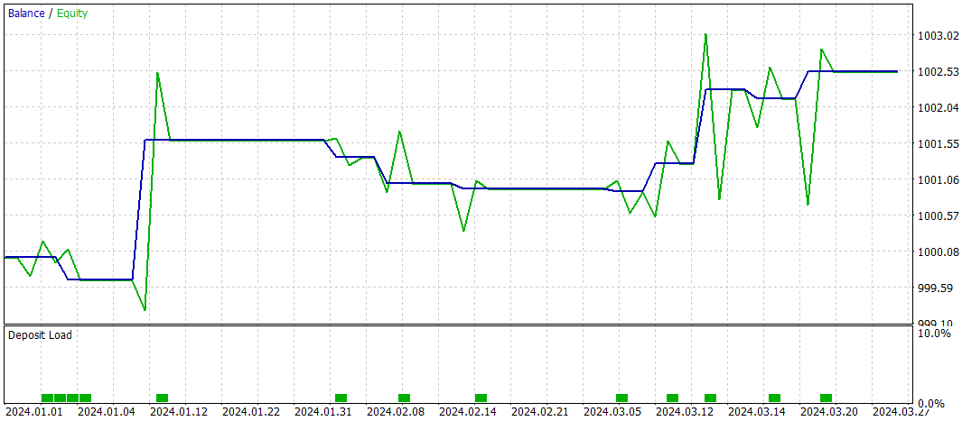

During the testing period, the model executed only 10 trades. This is a notably low frequency. Moreover, only 4 of these trades were profitable. Not an impressive result. However, both the average and maximum profit per winning trade were roughly five times greater than those of the losing trades. As a result, the model achieved a profit factor of 3.28.
In general, the model demonstrated a good profit-to-loss ratio, however, the limited number of trades suggests that we beed to increase trading frequency. Ideally without compromising trade quality.
Conclusion
Directional Diffusion Models (DDMs) offer a promising tool for the analysis and representation of market data in trading applications. Given that financial markets often exhibit anisotropic and directional patterns due to complex structural relationships and external macroeconomic drivers. Traditional diffusion models, based on isotropic processes, may fail to capture these nuances effectively. DDMs, on the other hand, adapt to the directionality of the data through the use of directional noise, enabling better identification of key patterns and trends even in high-noise, high-volatility environments.
In the practical part, we implemented our vision of the proposed approaches using MQL5. We trained the models on real historical market data and evaluated their performance on out-of-sample data. Based on the experimental results, we conclude that DDMs show strong potential. However, our current implementation still requires further optimization.
References
Programs used in the article
| # | Name | Type | Description |
|---|---|---|---|
| 1 | Research.mq5 | Expert Advisor | EA for collecting examples |
| 2 | ResearchRealORL.mq5 | Expert Advisor | EA for collecting examples using the Real-ORL method |
| 3 | Study.mq5 | Expert Advisor | Model training EA |
| 4 | Test.mq5 | Expert Advisor | Model testing EA |
| 5 | Trajectory.mqh | Class library | System state description structure |
| 6 | NeuroNet.mqh | Class library | A library of classes for creating a neural network |
| 7 | NeuroNet.cl | Library | OpenCL program code library |
Translated from Russian by MetaQuotes Ltd.
Original article: https://www.mql5.com/ru/articles/16269
Warning: All rights to these materials are reserved by MetaQuotes Ltd. Copying or reprinting of these materials in whole or in part is prohibited.
This article was written by a user of the site and reflects their personal views. MetaQuotes Ltd is not responsible for the accuracy of the information presented, nor for any consequences resulting from the use of the solutions, strategies or recommendations described.

- Free trading apps
- Over 8,000 signals for copying
- Economic news for exploring financial markets
You agree to website policy and terms of use