
Portfolio optimization in Forex: Synthesis of VaR and Markowitz theory

Introduction: Portfolio optimization tasks in Forex
I have spent the last three years developing trading robots for Forex. And you know what? Risk management is a real pain. At first, I just set fixed stops until I lost a couple of deposits. Then I started digging deeper and came across Markowitz's portfolio optimization theory.
It looked nice - you calculate correlations, optimize weights... But in reality this does not work very well for Forex. Why? Because in Forex all pairs are interrelated! Try trading EURUSD and EURGBP at the same time and you will see what I mean. One sharp EUR movement and both positions merge synchronously. A beautiful theory is shattered by harsh reality.
Having had enough of this, I started looking for other approaches. Eventually, I came across the Value at Risk (VaR) methodology. At first, I did not even understand what it was - some kind of complicated equations. But then it dawned on me - this is exactly what I needed! VaR shows the maximum loss for a given probability. In other words, we can directly estimate how much money we might lose in a day/week/month.
In the end, I decided to cross Markowitz with VaR. Sounds crazy? Maybe. But I did not see any other options. Markowitz provides the optimal allocation of funds, and VaR prevents from getting into a margin call. It looked great on paper.
Then began the harsh everyday life of a research programmer. Python, МetaТrader 5 terminal, tons of historical data... I knew it would not be easy, but reality exceeded all expectations. This is what I am going to tell you about – how I tried to create a system that actually works, and not just looks pretty in a backtest.
If you have ever tried to automate Forex trading, you will understand my pain. And if not, then maybe my experience will help you avoid at least some of the pitfalls you have to step on.
Theoretical and mathematical foundations of VaR and Markowitz theory
So, let's start with the theory. The first month I was just trying to get the hang of math. Markowitz's theory looks complicated - a bunch of equations, matrices, quadratic optimization... But in reality, everything is simple: you take the asset returns, calculate the correlations and find the weights so that the risk is minimal for a given return.
I was glad at first! But then I started testing on real Forex data, and then it all started... When using the history of EURUSD for a year, the distribution of returns was not normal at all. It was the same for GBPUSD. This is the key assumption in Markowitz's theory. In other words, all calculations go down the drain.
I spent a week looking for a solution. I dug through scientific articles, googled, read forums. I got back to my article about VaR - Value at Risk. It sounds smart, but in fact, we simply calculate how much we can lose with the probability of 95% (or whatever). First I tried the simplest option - parametric VaR. The equation is elementary: mean minus sigma per quantile. The operation quality is mediocre.
Then I switched to historical VaR. The idea is to take real history and look at what the losses were in the worst 5% of cases. This is much closer to reality, but a lot of data is needed. The final boss is the Monte Carlo method. We generate a bunch of random scenarios taking into account the correlations between pairs, and finally here we have something sensible.
The hardest part was figuring out how to combine VaR with Markowitz optimization. As a result, the following thing was born: we take standard optimization, but add a VaR limitation. We are looking for the minimum risk for a given return, but so that VaR does not exceed a certain level.
On paper everything is great, but we need to program it... In the following sections, I will show how I turned these equations into a working Python code.
Connecting to MetaTrader 5 from Python
The practical implementation of my system began with establishing a stable connection with the trading terminal. After experimenting with different approaches, I settled on a direct connection via the MetaTrader 5 library for Python, which turned out to be the most reliable and fast.
import MetaTrader5 as mt5
import time

def initialize_mt5(account=12345, server="MetaQuotes-Demo", password="abc123"):
    if not mt5.initialize():
        print(f"initialize() failed, error code = {mt5.last_error()}")
        return False

    authorized = mt5.login(account, password=password, server=server)
    if not authorized:
        print(f"login failed, error code = {mt5.last_error()}")
        mt5.shutdown()
        return False

    return True
A separate headache was synchronizing time between the broker server and the local system. A difference of a few seconds could lead to serious problems when calculating VaR. It was necessary to implement a special correction mechanism:
def get_time_correction():
    server_time = mt5.symbol_info_tick("EURUSD").time
    local_time = int(time.time())
    return server_time - local_time

def get_corrected_time():
    correction = get_time_correction()
    return int(time.time()) + correction
A lot of time was spent on optimizing data acquisition. Initially, I made requests for each currency pair separately, but after implementing batch processing, the speed increased several times:
def fetch_data_batch(symbols, timeframe, start_pos, count):
    data = {}
    for symbol in symbols:
        rates = mt5.copy_rates_from_pos(symbol, timeframe, start_pos, count)
        if rates is not None and len(rates) > 0:
            data[symbol] = rates
        else:
            print(f"Failed to get data for {symbol}")
            return None
    return data
It turned out to be surprisingly difficult to terminate the program correctly. It was necessary to develop a special 'graceful shutdown' procedure:
def safe_shutdown():
    try:
        positions = mt5.positions_get()
        if positions:
            for position in positions:
                close_position(position.ticket)

        orders = mt5.orders_get()
        if orders:
            for order in orders:
                mt5.order_send(request={"action": mt5.TRADE_ACTION_REMOVE,
                                      "order": order.ticket})
    finally:
        mt5.shutdown()
The result was a reliable foundation for the entire system, capable of operating around the clock without failures. It was already possible to build a more complex portfolio optimization logic on its basis. But this is already the topic of the next section.
Obtaining historical data and its pre-processing
Over the years of working with market data, I have learned one simple truth: the quality of historical data is critical to any trading system. Especially when it comes to portfolio optimization, where data errors can cascade.
I started by creating a reliable history loading system. The first version was quite simple, but practice quickly revealed its shortcomings. Quotes could contain gaps, spikes, and sometimes even outright incorrect values. Here is what the final code looks like for uploading with basic validation:
def load_historical_data(symbols, timeframe, start_date, end_date):
    data_frames = {}
    for symbol in symbols:
        # Load with a reserve to compensate for gaps
        rates = mt5.copy_rates_range(symbol, timeframe,
                                   start_date - timedelta(days=30),
                                   end_date)
        if rates is None:
            print(f"Failed to load data for {symbol}")
            continue

        df = pd.DataFrame(rates)
        df['time'] = pd.to_datetime(df['time'], unit='s')
        df.set_index('time', inplace=True)

        # Basic anomaly check
        df = detect_and_remove_spikes(df)
        df = fill_gaps(df)
        data_frames[symbol] = df

    return data_frames
A separate problem was handling gaps on weekends. At first I simply removed these days, but this distorted the volatility calculations. After long experiments, a method of interpolation was born, taking into account the specifics of each currency pair:
def fill_gaps(df, method='time'):
    if df.empty:
        return df

    # Check the intervals between points
    time_delta = df.index.to_series().diff()
    gaps = time_delta[time_delta > pd.Timedelta(hours=2)].index

    for gap_start in gaps:
        gap_end = df.index[df.index.get_loc(gap_start) + 1]
        # Create new points with interpolated values
        new_points = pd.date_range(gap_start, gap_end, freq='1H')[1:-1]

        for point in new_points:
            df.loc[point] = df.asof(point)

    return df.sort_index()
I tried several approaches to calculate returns. Simple percentage changes turned out to be too noisy. Logarithmic returns performed best in estimating VaR:
def calculate_returns(df):
    df['returns'] = np.log(df['close'] / df['close'].shift(1))
    df['rolling_std'] = df['returns'].rolling(window=20).std()
    df['rolling_mean'] = df['returns'].rolling(window=20).mean()

    # Clean out emissions using the 3-sigma rule
    mean = df['returns'].mean()
    std = df['returns'].std()
    df = df[abs(df['returns'] - mean) <= 3 * std]

    return df
The data verification system development turned out to be an important milestone. Each set undergoes a multi-stage check before being used in calculations:
def verify_data_quality(df, symbol):
    checks = {
        'missing_values': df.isnull().sum().sum() == 0,
        'price_continuity': (df['close'] > 0).all(),
        'timestamp_uniqueness': df.index.is_unique,
        'reasonable_returns': abs(df['returns']).max() < 0.1
    }

    if not all(checks.values()):
        failed_checks = [k for k, v in checks.items() if not v]
        print(f"Data quality issues for {symbol}: {failed_checks}")
        return False

    return True
I paid special attention to handling market anomalies. Various events, such as sharp movements due to the news or flash crashes, may greatly distort risk assessment. I have developed a special algorithm to identify and handle them correctly:
def detect_market_anomalies(df, window=20, threshold=3):
    volatility = df['returns'].rolling(window=window).std()
    typical_range = volatility.mean() + threshold * volatility.std()

    anomalies = df[abs(df['returns']) > typical_range].index
    if len(anomalies) > 0:
        print(f"Detected {len(anomalies)} market anomalies")

    return anomalies
The result was a reliable data handling pipeline that became the basis for all further calculations. Quality historical data is the foundation, without which it is impossible to build an efficient portfolio management system. In the next section, I will consider how this data is used to calculate VaR.
Implementation of VaR calculation for currency pairs
After a long time working with historical data, I delved into the implementation of VaR calculation. Initially, it seemed that it was enough to take ready-made equations and translate them into code. The reality turned out to be more complicated, since the specifics of Forex required serious modifications of standard approaches.
I started by implementing three classical VaR calculation methods. Here is what the parametric approach looks like:
def parametric_var(returns, confidence_level=0.95, holding_period=1):
    mu = returns.mean()
    sigma = returns.std()
    z_score = norm.ppf(1 - confidence_level)

    daily_var = -(mu + z_score * sigma)
    return daily_var * np.sqrt(holding_period)
However, it quickly became clear that the assumption of a normal distribution of returns in Forex often does not hold. The historical approach has proven to be more reliable:
def historical_var(returns, confidence_level=0.95, holding_period=1):
    sorted_returns = np.sort(returns)
    index = int((1 - confidence_level) * len(sorted_returns))
    daily_var = -sorted_returns[index]
    return daily_var * np.sqrt(holding_period)
But the most interesting results were provided by the Monte Carlo method. I modified it to take into account the specifics of the foreign exchange market:
def monte_carlo_var(returns, confidence_level=0.95, holding_period=1, simulations=10000):
    mu = returns.mean()
    sigma = returns.std()

    # Consider auto correlation of returns
    corr = returns.autocorr()

    simulated_returns = []
    for _ in range(simulations):
        daily_returns = []
        last_return = returns.iloc[-1]

        for _ in range(holding_period):
            # Generate the next value taking auto correlation into account
            innovation = np.random.normal(0, 1)
            next_return = mu + corr * (last_return - mu) + sigma * np.sqrt(1 - corr**2) * innovation
            daily_returns.append(next_return)
            last_return = next_return

        total_return = sum(daily_returns)
        simulated_returns.append(total_return)

    return -np.percentile(simulated_returns, (1 - confidence_level) * 100)
I paid special attention to the validation of the results. I also developed a backtesting system to check the VaR accuracy:
def backtest_var(returns, var, confidence_level=0.95):
    violations = (returns < -var).sum()
    expected_violations = len(returns) * (1 - confidence_level)

    z_score = (violations - expected_violations) / np.sqrt(expected_violations)
    p_value = 1 - norm.cdf(abs(z_score))

    return {
        'violations': violations,
        'expected': expected_violations,
        'z_score': z_score,
        'p_value': p_value
    }
To take into account the relationships between currency pairs, it was necessary to implement the calculation of portfolio VaR:
def portfolio_var(returns_df, weights, confidence_level=0.95, method='historical'):
    if method == 'parametric':
        portfolio_returns = returns_df.dot(weights)
        return parametric_var(portfolio_returns, confidence_level)

    elif method == 'historical':
        portfolio_returns = returns_df.dot(weights)
        return historical_var(portfolio_returns, confidence_level)

    elif method == 'monte_carlo':
        # Use the covariance matrix to generate
        # correlated random variables
        cov_matrix = returns_df.cov()
        L = np.linalg.cholesky(cov_matrix)

        means = returns_df.mean().values
        simulated_returns = []

        for _ in range(10000):
            Z = np.random.standard_normal(len(weights))
            R = means + L @ Z
            portfolio_return = weights @ R
            simulated_returns.append(portfolio_return)

        return -np.percentile(simulated_returns, (1 - confidence_level) * 100)
The result was a flexible VaR calculation system adapted to the specifics of Forex. In the next section, I will discuss how these calculations integrate with Markowitz theory for portfolio optimization.
Portfolio optimization using Markowitz method
After implementing a reliable VaR calculation, I began to focus on portfolio optimization. Markowitz's classical theory required serious adaptation to the realities of Forex. Months of experimentation and testing led me to several important discoveries.
The first thing I realized was that standard risk and return metrics work differently in Forex than they do in the stock market. Currency pairs have complex relationships that change over time. After much experimentation, I developed a modified expected return calculation function:
def calculate_expected_returns(returns_df, method='ewma', halflife=30):
    if method == 'ewma':
        # Exponentially weighted average gives more weight to recent data
        return returns_df.ewm(halflife=halflife).mean().iloc[-1]
    elif method == 'capm':
        # Modified CAPM for Forex
        risk_free_rate = 0.02  # annual risk-free rate
        market_returns = returns_df.mean(axis=1)  # market returns proxy
        betas = calculate_currency_betas(returns_df, market_returns)
        return risk_free_rate + betas * (market_returns.mean() - risk_free_rate)
The calculation of the covariance matrix also required some revision. The simple historical approach produced too unstable results. I implemented shrinkage estimation, which significantly improved the robustness of the optimization:
def shrinkage_covariance(returns_df, shrinkage_factor=None):
    sample_cov = returns_df.cov()
    n_assets = len(returns_df.columns)

    # The target matrix is diagonal with average variance
    target = np.diag(np.repeat(sample_cov.values.trace() / n_assets, n_assets))

    if shrinkage_factor is None:
        # Estimation of the optimal 'shrinkage' ratio
        shrinkage_factor = estimate_optimal_shrinkage(returns_df, sample_cov, target)

    shrunk_cov = (1 - shrinkage_factor) * sample_cov + shrinkage_factor * target
    return pd.DataFrame(shrunk_cov, index=sample_cov.index, columns=sample_cov.columns)
The hardest part is optimizing the portfolio weights. After many tests, I settled on a modified quadratic programming algorithm:
def optimize_portfolio(returns_df, expected_returns, covariance, target_return=None, constraints=None):
    n_assets = len(returns_df.columns)

    # Risk minimization function
    def portfolio_volatility(weights):
        return np.sqrt(weights.T @ covariance @ weights)

    # Limitations
    constraints = []
    # The sum of the weights is 1
    constraints.append({'type': 'eq', 'fun': lambda x: np.sum(x) - 1})

    if target_return is not None:
        # Target income limit
        constraints.append({
            'type': 'eq',
            'fun': lambda x: x @ expected_returns - target_return
        })

    # Add leverage restrictions for Forex
    constraints.append({
        'type': 'ineq',
        'fun': lambda x: 20 - np.sum(np.abs(x))  # max leverage 20
    })

    # Initial approximation - equal weights
    initial_weights = np.repeat(1/n_assets, n_assets)

    # Optimization
    result = minimize(
        portfolio_volatility,
        initial_weights,
        method='SLSQP',
        constraints=constraints,
        bounds=tuple((0, 1) for _ in range(n_assets))
    )

    if not result.success:
        raise OptimizationError("Failed to optimize portfolio: " + result.message)

    return result.x
I paid special attention to the problem of the solution stability. Small changes in input data should not lead to radical revision of the portfolio. For this purpose, I developed the regularization procedure:
def regularized_optimization(returns_df, current_weights, lambda_reg=0.1):
    # Add a penalty for deviation from the current weights
    def objective(weights):
        volatility = portfolio_volatility(weights)
        turnover_penalty = lambda_reg * np.sum(np.abs(weights - current_weights))
        return volatility + turnover_penalty
As a result, we have a reliable portfolio optimizer that takes into account the specifics of Forex and does not require frequent rebalancing. But the main thing was yet to come - combining this approach with a VaR-based risk control system.
Combining VaR and Markowitz into a single model
Combining the two approaches proved to be the most challenging part. I had to to find a way of using the advantages of both methods without creating contradictions between them. After several months of experimentation, I came up with an elegant solution.
The key idea was to use VaR as an additional constraint in the Markowitz optimization problem. Here's how it looks in the code:
def integrated_portfolio_optimization(returns_df, target_return, max_var_limit, current_weights=None):
    n_assets = len(returns_df.columns)

    # Calculation of basic metrics
    exp_returns = calculate_expected_returns(returns_df)
    covariance = shrinkage_covariance(returns_df)

    def objective_function(weights):
        # Portfolio standard deviation (Markowitz)
        portfolio_std = np.sqrt(weights.T @ covariance @ weights)

        # component VaR
        portfolio_var = calculate_portfolio_var(returns_df, weights)
        var_penalty = max(0, portfolio_var - max_var_limit)

        return portfolio_std + 100 * var_penalty  # Penalty for exceeding VaR
To take into account the dynamic nature of the market, I developed an adaptive system for recalculating parameters:
def adaptive_risk_limits(returns_df, base_var_limit, window=60):
    # Adapting VaR limits to current volatility
    recent_vol = returns_df.tail(window).std()
    long_term_vol = returns_df.std()
    vol_ratio = recent_vol / long_term_vol

    adjusted_var_limit = base_var_limit * np.sqrt(vol_ratio)
    return min(adjusted_var_limit, base_var_limit * 1.5)  # Limit growth
Particular attention had to be paid to the problem of solution stability. I have implemented a mechanism for smooth transition between portfolio states:
def smooth_rebalancing(old_weights, new_weights, max_change=0.1):
    weight_diff = new_weights - old_weights
    excess_change = np.abs(weight_diff) - max_change

    where_excess = excess_change > 0
    if where_excess.any():
        # Limit changes in weights
        adjustment = np.sign(weight_diff) * np.minimum(
            np.abs(weight_diff),
            np.where(where_excess, max_change, np.abs(weight_diff))
        )
        return old_weights + adjustment
    return new_weights
I developed a special metric to evaluate the efficiency of the combined approach:
def evaluate_integrated_model(returns_df, weights, var_limit):
    # Calculation of performance metrics
    portfolio_returns = returns_df.dot(weights)
    realized_var = historical_var(portfolio_returns)
    sharpe = calculate_sharpe_ratio(portfolio_returns)
    var_efficiency = abs(realized_var - var_limit) / var_limit

    return {
        'sharpe_ratio': sharpe,
        'var_efficiency': var_efficiency,
        'max_drawdown': calculate_max_drawdown(portfolio_returns),
        'turnover': calculate_turnover(weights)
    }
During the test, it turned out that the model works especially well during periods of increased volatility. The VaR component effectively limits risks, while Markowitz optimization continues to seek opportunities for profitability.
The final version of the system also includes a mechanism for automatic parameter adjustment:
def auto_tune_parameters(returns_df, initial_params, optimization_window=252):
    best_params = initial_params
    best_score = float('-inf')

    for var_limit in np.arange(0.01, 0.05, 0.005):
        for shrinkage in np.arange(0.2, 0.8, 0.1):
            params = {'var_limit': var_limit, 'shrinkage': shrinkage}
            score = backtest_model(returns_df, params, optimization_window)

            if score > best_score:
                best_score = score
                best_params = params

    return best_params
In the next section, I will discuss how this combined model is applied to dynamic position management in real trading.
Dynamic position sizing management
Translating the theoretical model into a practical trading system required solving many technical problems. The main one was the dynamic management of position sizes taking into account current market conditions and calculated optimal portfolio weights.
The basis of the system was a class for managing positions:
class PositionManager:
    def __init__(self, account_balance, risk_limit=0.02):
        self.balance = account_balance
        self.risk_limit = risk_limit
        self.positions = {}

    def calculate_position_size(self, symbol, weight, var_estimate):
        symbol_info = mt5.symbol_info(symbol)
        pip_value = symbol_info.trade_tick_value * 10

        # Calculate the position size taking into account VaR
        max_risk_amount = self.balance * self.risk_limit * abs(weight)
        position_size = max_risk_amount / (abs(var_estimate) * pip_value)

        # Round to minimum lot
        return round(position_size / symbol_info.volume_step) * symbol_info.volume_step
To smoothly change positions, I developed a mechanism of partial orders:
def adjust_positions(self, target_positions):
    for symbol, target_size in target_positions.items():
        current_size = self.get_current_position(symbol)
        if abs(target_size - current_size) > self.min_adjustment:
            # Break big changes into pieces
            steps = min(5, int(abs(target_size - current_size) / self.min_adjustment))
            step_size = (target_size - current_size) / steps

            for i in range(steps):
                next_size = current_size + step_size
                self.execute_order(symbol, next_size - current_size)
                current_size = next_size
                time.sleep(1)  # Prevent order flooding
I paid special attention to risk control when changing positions:
def execute_order(self, symbol, size_delta, max_slippage=10):
    if size_delta > 0:
        order_type = mt5.ORDER_TYPE_BUY
    else:
        order_type = mt5.ORDER_TYPE_SELL

    # Get current prices
    tick = mt5.symbol_info_tick(symbol)

    # Set VaR-based stop loss
    if order_type == mt5.ORDER_TYPE_BUY:
        stop_loss = tick.bid - (self.var_estimates[symbol] * tick.bid)
        take_profit = tick.bid + (self.var_estimates[symbol] * 2 * tick.bid)
    else:
        stop_loss = tick.ask + (self.var_estimates[symbol] * tick.ask)
        take_profit = tick.ask - (self.var_estimates[symbol] * 2 * tick.ask)

    request = {
        "action": mt5.TRADE_ACTION_DEAL,
        "symbol": symbol,
        "volume": abs(size_delta),
        "type": order_type,
        "price": tick.ask if order_type == mt5.ORDER_TYPE_BUY else tick.bid,
        "sl": stop_loss,
        "tp": take_profit,
        "deviation": max_slippage,
        "magic": 234000,
        "comment": "var_based_adjustment",
        "type_time": mt5.ORDER_TIME_GTC,
        "type_filling": mt5.ORDER_FILLING_IOC,
    }

    result = mt5.order_send(request)
    return self.handle_order_result(result)
I added a volatility monitoring system to protect against sharp market movements:
def monitor_volatility(self, returns_df, threshold=2.0):
    # Current volatility calculation
    current_vol = returns_df.tail(20).std() * np.sqrt(252)
    historical_vol = returns_df.std() * np.sqrt(252)

    if current_vol > historical_vol * threshold:
        # Reduce positions in case of increased volatility
        self.reduce_exposure(current_vol / historical_vol)
        return False

    return True
The system also includes a mechanism for automatically closing positions when critical risk levels are reached:
def emergency_close(self, max_loss_percent=5.0):
    total_loss = sum(pos.profit for pos in mt5.positions_get())
    if total_loss < -self.balance * max_loss_percent / 100:
        print("Emergency closure triggered!")
        for position in mt5.positions_get():
            self.close_position(position.ticket)
The result is a robust position management system that can operate effectively in a variety of market conditions. The next section will focus on the VaR-based risk control system.
Portfolio risk control system
After implementing dynamic position management, I was faced with the need to create a comprehensive risk control system at the portfolio level. Experience has shown that local risk control of individual positions is not sufficient – a holistic approach is needed.
I started with the creation of a class for monitoring portfolio risks:
class PortfolioRiskManager:
    def __init__(self, max_portfolio_var=0.03, max_correlation=0.7, max_drawdown=0.1):
        self.max_portfolio_var = max_portfolio_var
        self.max_correlation = max_correlation
        self.max_drawdown = max_drawdown
        self.current_drawdown = 0
        self.peak_balance = 0

    def update_portfolio_metrics(self, positions, returns_df):
        # Calculation of current portfolio weights
        total_exposure = sum(abs(pos.volume) for pos in positions)
        weights = {pos.symbol: pos.volume/total_exposure for pos in positions}

        # Update portfolio VaR
        self.current_var = self.calculate_portfolio_var(returns_df, weights)

        # Check correlations
        self.check_correlations(returns_df, weights)
I paid special attention to monitoring correlations between instruments:
def check_correlations(self, returns_df, weights):
    corr_matrix = returns_df.corr()
    high_corr_pairs = []

    for i in returns_df.columns:
        for j in returns_df.columns:
            if i < j and abs(corr_matrix.loc[i,j]) > self.max_correlation:
                if weights.get(i, 0) > 0 and weights.get(j, 0) > 0:
                    high_corr_pairs.append((i, j, corr_matrix.loc[i,j]))

    if high_corr_pairs:
        self.handle_high_correlations(high_corr_pairs, weights)
I implemented dynamic risk management depending on market conditions:
def adjust_risk_limits(self, market_state):
    volatility_factor = market_state.get('volatility_ratio', 1.0)
    trend_strength = market_state.get('trend_strength', 0.5)

    # Adapt limits to market conditions
    self.max_portfolio_var *= np.sqrt(volatility_factor)
    if trend_strength > 0.7:  # Strong trend
        self.max_drawdown *= 1.2  # Allow a big drawdown
    elif trend_strength < 0.3:  # Weak trend
        self.max_drawdown *= 0.8  # Reduce the acceptable drawdown
The drawdown monitoring system turned out to be particularly interesting:
def monitor_drawdown(self, current_balance):
    if current_balance > self.peak_balance:
        self.peak_balance = current_balance

    self.current_drawdown = (self.peak_balance - current_balance) / self.peak_balance

    if self.current_drawdown > self.max_drawdown:
        return self.handle_excessive_drawdown()
    elif self.current_drawdown > self.max_drawdown * 0.8:
        return self.reduce_risk_exposure(0.8)

    return True
I added a stress test system to protect against extreme events:
def stress_test_portfolio(self, returns_df, weights, scenarios=1000):
    results = []

    for _ in range(scenarios):
        # Simulate extreme conditions
        stress_returns = returns_df.copy()

        # Increase volatility
        vol_multiplier = np.random.uniform(1.5, 3.0)
        stress_returns *= vol_multiplier

        # Add random shocks
        shock_magnitude = np.random.uniform(-0.05, 0.05)
        stress_returns += shock_magnitude

        # Calculate losses in a stress scenario
        portfolio_return = (stress_returns * weights).sum(axis=1)
        results.append(portfolio_return.min())

    return np.percentile(results, 1)  # 99% VaR in case of a stress
The result is a multi-level capital protection system that effectively prevents excessive risks and helps to survive periods of high volatility. In the next section, I will discuss how all of these components work together in real trading.
Visualizing analysis results
Visualization became an important stage of my research. After implementing all the calculation modules, it was necessary to create a visual representation of the results. I have developed several key graphical components that help monitor the system's performance in real time.
I started with visualizing the portfolio structure and its evolution:
def plot_portfolio_composition(weights_history):
    plt.figure(figsize=(15, 8))
    ax = plt.gca()

    # Create a graph of weight changes over time
    dates = weights_history.index
    bottom = np.zeros(len(dates))

    for symbol in weights_history.columns:
        plt.fill_between(dates, bottom, bottom + weights_history[symbol],
                        label=symbol, alpha=0.6)
        bottom += weights_history[symbol]

    plt.title('Evolution of portfolio structure')
    plt.legend(bbox_to_anchor=(1.05, 1), loc='upper left')
    plt.grid(True, alpha=0.3)
Particular attention was paid to visualizing risks. I also developed a VaR heat map for different currency pairs:
def plot_var_heatmap(var_matrix):
    plt.figure(figsize=(12, 8))
    sns.heatmap(var_matrix, annot=True, cmap='RdYlBu_r',
                fmt='.2%', center=0)
    plt.title('Portfolio risk map (VaR)')

    # Add a timestamp
    plt.annotate(f'Last update: {datetime.now().strftime("%Y-%m-%d %H:%M")}',
                xy=(0.01, -0.1), xycoords='axes fraction')
To analyze profitability, I created an interactive chart with important events highlighted:
def plot_performance_analytics(returns_df, var_values, significant_events):
    fig = plt.figure(figsize=(15, 10))
    gs = GridSpec(2, 1, height_ratios=[3, 1])

    # Returns graph
    ax1 = plt.subplot(gs[0])
    cumulative_returns = (1 + returns_df).cumprod()
    ax1.plot(cumulative_returns.index, cumulative_returns,
             label='Portfolio returns')

    # Mark important events
    for date, event in significant_events.items():
        ax1.axvline(x=date, color='r', linestyle='--', alpha=0.3)
        ax1.annotate(event, xy=(date, ax1.get_ylim()[1]),
                    xytext=(10, 10), textcoords='offset points',
                    rotation=45)

    # VaR graph
    ax2 = plt.subplot(gs[1])
    ax2.fill_between(var_values.index, -var_values,
                     color='lightblue', alpha=0.5,
                     label='Value at Risk')
I added an interactive dashboard to monitor the portfolio status:
class PortfolioDashboard:
    def __init__(self):
        self.fig = plt.figure(figsize=(15, 10))
        self.setup_subplots()

    def setup_subplots(self):
        gs = self.fig.add_gridspec(3, 2)
        self.ax_returns = self.fig.add_subplot(gs[0, :])
        self.ax_weights = self.fig.add_subplot(gs[1, 0])
        self.ax_risk = self.fig.add_subplot(gs[1, 1])
        self.ax_metrics = self.fig.add_subplot(gs[2, :])

    def update(self, portfolio_data):
        self._plot_returns(portfolio_data['returns'])
        self._plot_weights(portfolio_data['weights'])
        self._plot_risk_metrics(portfolio_data['risk'])
        self._update_metrics_table(portfolio_data['metrics'])

        plt.tight_layout()
        plt.show()
I developed a dynamic visualization to analyze correlations:
def plot_correlation_dynamics(returns_df, window=60):
    # Calculation of dynamic correlations
    correlations = returns_df.rolling(window=window).corr()

    # Create an animated graph
    fig, ax = plt.subplots(figsize=(10, 10))

    def update(frame):
        ax.clear()
        sns.heatmap(correlations.loc[frame],
                    vmin=-1, vmax=1, center=0,
                    cmap='RdBu', ax=ax)
        ax.set_title(f'Correlations on {frame.strftime("%Y-%m-%d")}')
All these visualizations help to quickly assess the state of the portfolio and make trading decisions. In the next section, I will test the system.
Strategy backtesting
After completing the development of all components of the system, I was faced with the need for its thorough testing. The process turned out to be much more complicated than simply running historical data. It was necessary to take into account many factors: slippage, commissions, and the specifics of order execution at different brokers.
Initial backtesting attempts showed that the classic approach with fixed spreads yields overly optimistic results. It was necessary to create a more realistic model that takes into account the change in spreads depending on volatility and time of day.
I paid special attention to modeling data gaps and liquidity issues. In real trading, situations often arise when an order cannot be executed at the estimated price. These scenarios must be handled correctly during testing.
Here is the complete implementation of the backtesting system:
class PortfolioBacktester:
    def __init__(self, initial_capital=100000, commission=0.0001):
        self.initial_capital = initial_capital
        self.commission = commission
        self.positions = {}
        self.trades_history = []
        self.balance_history = []
        self.var_history = []
        self.metrics = {}

    def run_backtest(self, returns_df, optimization_params):
        self.current_capital = self.initial_capital
        portfolio_returns = []

        # Preparing sliding windows for calculations
        window = 252  # Trading yesr
        for i in range(window, len(returns_df)):
            # Receive historical data for calculation
            historical_returns = returns_df.iloc[i-window:i]

            # Optimize the portfolio
            weights = self.optimize_portfolio(
                historical_returns,
                optimization_params['target_return'],
                optimization_params['max_var']
            )

            # Calculate VaR for the current distribution
            current_var = self.calculate_portfolio_var(
                historical_returns,
                weights,
                optimization_params['confidence_level']
            )

            # Check the need for rebalancing
            if self.should_rebalance(weights, current_var):
                self.execute_rebalancing(weights, returns_df.iloc[i])

            # Update positions and calculate profitability
            portfolio_return = self.update_positions(returns_df.iloc[i])
            portfolio_returns.append(portfolio_return)

            # Update metrics
            self.update_metrics(portfolio_return, current_var)

            # Check stop losses triggering
            self.check_stop_losses(returns_df.iloc[i])

        # Calculate the final metrics
        self.calculate_final_metrics(portfolio_returns)

    def optimize_portfolio(self, returns, target_return, max_var):
        # Using our hybrid optimization model
        opt = HybridOptimizer(returns, target_return, max_var)
        weights = opt.optimize()
        return self.apply_position_limits(weights)

    def execute_rebalancing(self, target_weights, current_prices):
        for symbol, target_weight in target_weights.items():
            current_weight = self.get_position_weight(symbol)
            if abs(target_weight - current_weight) > self.REBALANCING_THRESHOLD:
                # Simulate execution with slippage
                slippage = self.simulate_slippage(symbol, current_prices[symbol])
                trade_price = current_prices[symbol] * (1 + slippage)

                # Calculate the deal size
                trade_volume = self.calculate_trade_volume(
                    symbol, current_weight, target_weight
                )

                # Consider commissions
                commission = abs(trade_volume * trade_price * self.commission)
                self.current_capital -= commission

                # Set a deal to history
                self.record_trade(symbol, trade_volume, trade_price, commission)

    def update_metrics(self, portfolio_return, current_var):
        self.balance_history.append(self.current_capital)
        self.var_history.append(current_var)

        # Updating performance metrics
        self.metrics['max_drawdown'] = self.calculate_drawdown()
        self.metrics['sharpe_ratio'] = self.calculate_sharpe()
        self.metrics['var_efficiency'] = self.calculate_var_efficiency()

    def calculate_final_metrics(self, portfolio_returns):
        returns_series = pd.Series(portfolio_returns)

        self.metrics['total_return'] = (self.current_capital / self.initial_capital - 1)
        self.metrics['volatility'] = returns_series.std() * np.sqrt(252)
        self.metrics['sortino_ratio'] = self.calculate_sortino(returns_series)
        self.metrics['calmar_ratio'] = self.calculate_calmar()
        self.metrics['var_breaches'] = self.calculate_var_breaches()

    def simulate_slippage(self, symbol, price):
        # Simulate realistic slippage
        base_slippage = 0.0001  # Basic slippage
        time_factor = self.get_time_factor()  # Time dependency
        volume_factor = self.get_volume_factor(symbol)  # Volume dependency

        return base_slippage * time_factor * volume_factor
The test results were quite revealing. The hybrid model demonstrated significantly better resilience to market shocks compared to classical approaches. This was especially evident during periods of high volatility, when the VaR limit effectively protected the portfolio from excess risks.
Final debugging
After many months of development and testing, I finally arrived at the final version of the system. To be honest, it is very different from what I originally planned. Practice forced many changes, some of which were quite unexpected.
The first major change was in the way I handled data. I realized that testing the system only on historical data was not enough - it was necessary to check its behavior in a wide variety of market conditions. So I developed a system for generating synthetic data. It sounds simple, but in reality it took several weeks.
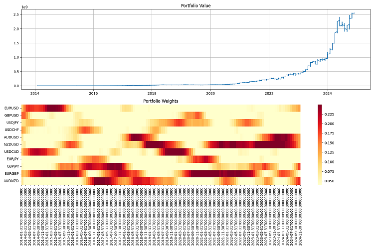
I started by dividing all currency pairs into groups based on liquidity. The first group included major pairs, such as EURUSD and GBPUSD. The second one contained commodity currency pairs, such as AUDUSD and USDCAD. Next came the crosses - EURJPY, GBPJPY and others. Finally, there were exotic pairs, like CADJPY and EURAUD. For each group, I set my own volatility and correlation parameters, as close to real ones as possible.
But the most interesting thing started when I added different market modes. Imagine: a third of the time the market is calm, the volatility is low. Another third is normal trade. And the remaining time is increased volatility, when everything flies like crazy. Besides, I added long-term trends and cyclical fluctuations. It turned out to be very similar to the real market.
Portfolio optimization also required some effort. At first I thought to get by with simple restrictions on the weights of positions, but I quickly realized that this was not enough. So, I added dynamic risk premiums - the higher the volatility of the pair, the higher the potential return should be. Introduced restrictions: minimum - 4% per position, maximum - 25%. It seems like a lot, but if you have leverage, it is normal.
Speaking of the leverage. This is a separate story. At first, I played it safe and worked almost without it. But analysis showed that moderate leverage, around 10 to 1, significantly improved results. The main thing is to take into account all costs correctly. And there are quite a few of them: trade commissions (two basis points), leverage maintenance interest (0.01% per day), execution slippage. All this had to be built into the optimizer.
A separate headache is protection from margin calls. After several unsuccessful experiments, I settled on a simple solution: if the drawdown exceeds 10%, close all positions and save at least part of the capital. It sounds conservative, but works great in the long run.
The most difficult thing was reporting. When your system works with dozens of currency pairs and constantly buys and sells something, it is simply impossible to keep track of everything. I had to develop a whole monitoring system: annual reports with a bunch of metrics, graphs of everything and anything: from the simple value of the portfolio to heat maps of the distribution of weights.
I conducted the final testing over a long period - from 2000 to 2024. I took a million dollars as initial capital and rebalanced it once a quarter. I was pleased with the results. The system adapts well to different market conditions and keeps risks under control. Even in the most severe crises, it manages to preserve most of its capital.
But there is still a lot of work to do. I would like to add machine learning to predict volatility. Currently, the system only works with historical data. Besides, I am thinking about how to make leverage management more flexible. Rebalancing frequency could be optimized as well. Sometimes a quarter is too long, while sometimes you can leave positions alone for six months.
In general, it turned out completely different from what I originally planned. But, as they say, the best is the enemy of the good. The system works, controls risks, and makes money. And this is the main thing.
Conclusion
That was a cool ride. When I first started messing around with Markowitz's theory, I could not even imagine what it would turn into. I just wanted to apply a conventional approach to Forex, but in the end I had to invent some kind of Frankenstein's monster from different approaches to risk management.
The coolest thing is that I managed to cross Markowitz with VaR, and this thing really works! The funny thing is that both methods proved to be mediocre separately, but together they give excellent results. I was especially pleased with how the system holds up when the market is shaking. VaR is simply amazing as a limiter in optimization.
Of course, I had a lot of trouble with the technical part. But now everything is taken into account: slippage, commissions, and execution features.
I tested the system on historical data from 2000 to 2024. The results were pretty good. It adapts well to different market conditions and does not even collapse during crises. With a leverage of 10 to 1 it works like clockwork. The main thing is to control the risks rigidly.
But there is still a ton of work to do. I would like to:
- add machine learning to volatility forecasts (this will be the topic of the next article);
- sort out rebalancing frequency - maybe it can be optimized;
- make leverage management smarter (dynamic leverage and dynamic "smart" deposit loading will also be implemented in future articles);
- train the system to adapt even better to different market regimes.
In general, the main conclusion is this: a cool trading system is not just equations from a textbook. Here you need to understand the market, be savvy in technology, and it is especially important to be able to keep risks in check. All these developments can now be applied to other markets, not only to Forex. Although there is still room for growth, the foundation is already there, and it works.
Translated from Russian by MetaQuotes Ltd.
Original article: https://www.mql5.com/ru/articles/16604
Warning: All rights to these materials are reserved by MetaQuotes Ltd. Copying or reprinting of these materials in whole or in part is prohibited.
This article was written by a user of the site and reflects their personal views. MetaQuotes Ltd is not responsible for the accuracy of the information presented, nor for any consequences resulting from the use of the solutions, strategies or recommendations described.


- Free trading apps
- Over 8,000 signals for copying
- Economic news for exploring financial markets
You agree to website policy and terms of use