Neural Networks in Trading: Node-Adaptive Graph Representation with NAFS

Introduction

In recent years, graph representation learning has been widely applied in various application scenarios such as node clustering, link prediction, node classification, and graph classification. The goal of graph representation learning is to encode graph information into node embeddings. Traditional methods for graph representation learning have primarily focused on preserving information about the graph structure. However, these methods face two major limitations:

1. Shallow architecture. While Graph Convolutional Networks (GCNs) employ multiple layers to capture deep structural information, increasing the number of layers often leads to over-smoothing, resulting in indistinguishable node embeddings.
2. Poor scalability. GNN-based graph representation learning methods may fail to scale to large graphs due to high computational costs and significant memory consumption.

The authors of the paper "NAFS: A Simple yet Tough-to-beat Baseline for Graph Representation Learning" set out to address these issues by introducing a novel graph representation method based on simple feature smoothing followed by adaptive combination. The Node-Adaptive Feature Smoothing (NAFS) method generates superior node embeddings by integrating both the graph's structural information and node features. Based on the observation that different nodes exhibit highly varied "smoothing speeds", NAFS adaptively smooths each node's features, using both low- and high-order neighborhood information. Furthermore, feature ensembles are used to combine smoothed features extracted using different smoothing operators. Since NAFS requires no training, it significantly reduces training costs and scales efficiently to large graphs.

1. The NAFS Algorithm

Many researchers have proposed separating feature smoothing and transformation within each GCN layer to enable scalable node classification. Specifically, they first apply feature smoothing operations in a preprocessing step, and then feed the processed features into a simple MLP to produce final node label predictions.

Such decoupled GNNs consist of two parts: feature smoothing and MLP training. The feature smoothing phase combines structural graph information with node features to generate more informative inputs for the subsequent MLP. During training, the MLP only learns from these smoothed features.

Another branch of GNN research also separates smoothing and transformation but follows a different approach. Raw node features are first fed into an MLP to generate intermediate embeddings. This is followed by personalized propagation operations applied to these embeddings to obtain final predictions. However, this GNN branch still needs to perform recursive propagation operations in each training epoch, making it impractical for large-scale graphs.

The simplest way to capture rich structural information is to stack multiple GNN layers. However, repeated feature smoothing in GNN models leads to indistinguishable node embeddings - the well-known over-smoothing problem.

Quantitative analysis empirically shows that a node's degree plays a significant role in determining its optimal smoothing step. Intuitively, high-degree nodes should undergo fewer smoothing steps compared to low-degree nodes.

While applying feature smoothing within decoupled GNNs enables scalable training for large graphs, indiscriminate smoothing across all nodes results in suboptimal embeddings. Nodes with different structural properties require different smoothing rates. Therefore, node-adaptive feature smoothing should be used to satisfy each node's unique smoothing requirements.

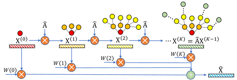
When applied sequentially, 𝐗l=Â𝐗l−1, the smoothed node embedding matrix 𝐗l−1 accumulates a deeper structural information as l increases. The multi-scale node embedding matrices {𝐗0, 𝐗1, …, 𝐗K} (where K is the maximum smoothing step) are then merged into a unified matrix Ẋ that combines both local and global neighborhood information.

The NAFS authors' analysis shows that the rate at which each node reaches a steady state varies greatly. Therefor, individualized node analysis is required. To this end, NAFS introduces the concept of smoothing weight, calculated based on the distance between a node's local and smoothed feature vectors. This allows the smoothing process to be tailored individually for each node.

A more effective alternative involves replacing the smoothing matrix  with cosine similarity. A higher cosine similarity between a node’s local and smoothed feature vectors indicates that node vi is further from equilibrium, and that [Âk𝐗]i intuitively contains mire up-to-date information. Thus, for node vi, smoothed features with higher cosine similarity should contribute more to its final embedding.

Different smoothing operators effectively act as distinct knowledge extractors. This enables the capture of graph structures across various scales and dimensions. To achieve this, feature ensemble operations use multiple knowledge extractors. These extractors are used within the feature smoothing process to generate diverse smoothed features.

NAFS produces node embeddings without any training, making it highly efficient and scalable. Moreover, the node-adaptive feature smoothing strategy allows for capturing deep structural information.

The authors' visualization of the NAFS method is shown below.

2. Implementation in MQL5

After covering the theoretical aspects of the NAFS framework, we now move on to its practical implementation using MQL5. Before we proceed to the actual implementation, let's clearly outline the main stages of the framework.

1. Constructing the multi-scale node representation matrix.
2. Calculating smoothing weights based on cosine similarity between the node's feature vector and its smoothed representations.
3. Computing the weighted average for the final embedding.

It's worth noting that some of these operations can be implemented using the existing functionality of our library. For example, calculating cosine similarity and computing weighted averages can be efficiently implemented via matrix multiplication. The Softmax layer can assist in determining the smoothing coefficients.

The remaining question is constructing the multi-scale node representation matrix.

2.1 Multi-Scale Node Representation Matrix

To construct the multi-scale node representation matrix, we will use a simple averaging of individual node features with the corresponding features of its immediate neighbors. Multi-scale behavior is achieved by applying averaging windows of varying sizes.

In our works, we implements major computations in the OpenCL context. Consequently, the matrix construction process will also be delegated to parallel computing. For this purpose, we will create a new kernel in the OpenCL program FeatureSmoothing.

__kernel void FeatureSmoothing(__global const float *feature,
                               __global float *outputs,
                               const int smoothing
                              )
  {
   const size_t pos = get_global_id(0);
   const size_t d = get_global_id(1);
   const size_t total = get_global_size(0);
   const size_t dimension = get_global_size(1);

In the kernel parameters, we receive pointers to two data buffers (the source data and the results), along with a constant specifying the number of smoothing scales. In this case, we do not define a specific smoothing scale step size, as it is assumed to be "1". The averaging window expands by 2 elements. Because we equally extend it both before and after the target element.

It is important to note that the number of smoothing scales cannot be negative. If this value is zero, we simply pass the source data through unchanged.

We plan to execute this kernel in a two-dimensional task space consisting of fully independent threads, without creating local workgroups. The first dimension corresponds to the size of the source sequence being analyzed, while the second dimension represents the number of features in the vector describing each sequence element.

Within the kernel body, we immediately identify the current thread by all dimensions of the task space and determine their respective sizes.

Using the obtained data, we calculate the offsets within the data buffers.

   const int shift_input = pos * dimension + d;
   const int shift_output = dimension * pos * smoothing + d;

At this point, the preparatory stage is complete, and we proceed directly to generating the multi-scale representations. The first step is to copy the source data, which corresponds to the representation at zero-level averaging.

   float value = feature[shift_input];
   if(isinf(value) || isnan(value))
      value = 0;
   outputs[shift_output] = value;

Next, we organize a loop to compute the mean values of individual features within the averaging window. As you can imagine, this requires summing all values within the window, followed by dividing the accumulated sum by the number of elements included in the summation.

It is important to note that all averaging windows for different scales are centered around the same element under analysis. Consequently, each subsequent scale incorporates all elements from the previous scale. We take advantage of this property to minimize accesses to expensive global memory: at each iteration, we only add the newly included values to the previously accumulated sum, and then divide the current accumulated sum by the number of elements in the current averaging window.

   for(int s = 1; s <= smoothing; s++)
     {
      if((pos - s) >= 0)
        {
         float temp = feature[shift_input - s * dimension];
         if(isnan(temp) || isinf(temp))
            temp = 0;
         value += temp;
        }
      if((pos + s) < total)
        {
         float temp = feature[shift_input + s * dimension];
         if(isnan(temp) || isinf(temp))
            temp = 0;
         value += temp;
        }
      float factor = 1.0f / (min((int)total, (int)(pos + s)) - max((int)(pos - s), 0) + 1);
      if(isinf(value) || isnan(value))
         value = 0;
      float out = value * factor;
      if(isinf(out) || isnan(out))
         out = 0;
      outputs[shift_output + s * dimension] = out;
     }
  }

It is also worth mentioning (although it may sound somewhat counterintuitive) that not all averaging windows within the same scale have the same size. This is due to edge elements in the sequence, where the averaging window extends beyond the sequence boundaries on either side. Therefore, at each iteration, we calculate the actual number of elements involved in the averaging.

In a similar manner, we construct the error gradient propagation algorithm through the above-described operations in the FeatureSmoothingGradient kernel, which I suggest you review independently. The full OpenCL program code can be found in the attachment.

2.2 Building the NAFS Class

After making the necessary additions to the OpenCL program, we move on to the main application, where we will create a new class for adaptive node embedding formation: CNeuronNAFS. The structure of the new class is shown below.

class CNeuronNAFS :  public CNeuronBaseOCL
  {
protected:
   uint                 iDimension;
   uint                 iSmoothing;
   uint                 iUnits;
   //---
   CNeuronBaseOCL       cFeatureSmoothing;
   CNeuronTransposeOCL  cTranspose;
   CNeuronBaseOCL       cDistance;
   CNeuronSoftMaxOCL    cAdaptation;
   //---
   virtual bool      FeatureSmoothing(const CNeuronBaseOCL *neuron, const CNeuronBaseOCL *smoothing);
   virtual bool      FeatureSmoothingGradient(const CNeuronBaseOCL *neuron, const CNeuronBaseOCL *smoothing);
   //---
   virtual bool      feedForward(CNeuronBaseOCL *NeuronOCL) override;
   virtual bool      calcInputGradients(CNeuronBaseOCL *NeuronOCL) override;
   virtual bool      updateInputWeights(CNeuronBaseOCL *NeuronOCL) override { return true; }

public:
                     CNeuronNAFS(void) {};
                    ~CNeuronNAFS(void) {};
   //---
   virtual bool      Init(uint numOutputs, uint myIndex, COpenCLMy *open_cl,
                          uint window, uint step, uint units_count,
                          ENUM_OPTIMIZATION optimization_type, uint batch);
   //---
   virtual int       Type(void) override   const   {  return defNeuronNAFS; }
   //---
   virtual bool      Save(int const file_handle) override;
   virtual bool      Load(int const file_handle) override;
   //---
   virtual bool      WeightsUpdate(CNeuronBaseOCL *source, float tau) override;
   virtual void      SetOpenCL(COpenCLMy *obj) override;
  };

As can be seen, the structure of the new class declares three variables and four internal layers. We will review their functionality during the implementation of the algorithms within the overridden virtual methods.

We also have two wrapper methods for the identically named kernels in the OpenCL program described earlier. They are built using the standard kernel calling algorithm. You can find the code them yourself in the attachment.

All internal objects of the new class are declared statically, allowing us to leave the class constructor and destructor "empty". The initialization of these declared and inherited objects is performed in the Init method.

bool CNeuronNAFS::Init(uint numOutputs, uint myIndex, COpenCLMy *open_cl,
                       uint dimension, uint smoothing, uint units_count,
                       ENUM_OPTIMIZATION optimization_type, uint batch)
  {
   if(!CNeuronBaseOCL::Init(numOutputs, myIndex, open_cl, dimension * units_count,
                            optimization_type, batch))
      return false;

In the method parameters, we receive the main constants that allow us to uniquely determine the architecture of the object being created. These include:

• dimension – the size of the feature vector describing a single sequence element;
• smoothing – the number of smoothing scales (if set to zero, the source data is copied directly);
• units_count – the size of the sequence being analyzed.

Note that all parameters are of unsigned integer type. This approach eliminates the possibility of receiving negative parameter values. 

Inside the method, as usual, we first call the parent class method of the same name, which already handles parameter validation and initialization of inherited objects. The size of the result tensor is assumed to match the size of the input tensor and is calculated as the product of the number of elements in the analyzed sequence and the size of the feature vector for a single element.

After successful execution of the parent class method, we save the externally provided parameters into internal variables with corresponding names.

   iDimension = dimension;
   iSmoothing = smoothing;
   iUnits = units_count;

Next, we move on to initializing the declared objects. First, we declare the internal layer for storing the multi-scale node representation matrix. Its size must be sufficient to store the complete matrix. Therefore, it is (iSmoothing + 1) times larger than the size of the original data.

   if(!cFeatureSmoothing.Init(0, 0, OpenCL, (iSmoothing + 1) * iUnits * iDimension, optimization, iBatch))
      return false;
   cFeatureSmoothing.SetActivationFunction(None);

After constructing the multi-scale node representations (in our case, these represent candlestick patterns at various scales), we need to calculate the cosine similarity between these representations and the feature vector of the analyzed bar. To do this, we multiply the input tensor by the multi-scale node representation tensor. However, prior to performing this multiplication, we must first transpose the multi-scale representation tensor.

   if(!cTranspose.Init(0, 1, OpenCL, (iSmoothing + 1)*iUnits, iDimension, optimization, iBatch))
      return false;
   cTranspose.SetActivationFunction(None);

The matrix multiplication operation has already been implemented in our base neural layer class and inherited from the parent class. To save the results of this operation, we initialize the internal object cDistance.

   if(!cDistance.Init(0, 2, OpenCL, (iSmoothing + 1)*iUnits, optimization, iBatch))
      return false;
   cDistance.SetActivationFunction(None);

Let me remind you that multiplying two vectors pointing in the same direction yields positive values, while opposite directions yield negative values. Clearly, if the analyzed bar aligns with the overall trend, the multiplication result between the bar's feature vector and the smoothed values will be positive. Conversely, if the bar opposes the general trend, the result will be negative. In flat market conditions, the smoothed value vector will be close to zero. Consequently, the multiplication result will also approach zero. To normalize the resulting values and calculate the adaptive influence coefficients for each scale, we use the Softmax function.

   if(!cAdaptation.Init(0, 3, OpenCL, cDistance.Neurons(), optimization, iBatch))
      return false;
   cAdaptation.SetActivationFunction(None);
   cAdaptation.SetHeads(iUnits);

Now, to compute the final embedding for the analyzed node (bar), we multiply the adaptive coefficient vector of each node by the corresponding multi-scale representation matrix. The result of this operation is written to the buffer of the interface for data exchange with the subsequent layer inherited from the parent class. Therefore, we do not create an additional internal object. Instead, we simply disable the activation function and complete the initialization method, returning the logical result of the operation to the calling program.

   SetActivationFunction(None);
//---
   return true;
  }

After completing the work on initializing the new object, we move on to constructing feed-forward pass algorithms in the feedForward method. In the method parameters, we receive a pointer to the source data object.

bool CNeuronNAFS::feedForward(CNeuronBaseOCL *NeuronOCL)
  {
   if(!FeatureSmoothing(NeuronOCL, cFeatureSmoothing.AsObject()))
      return false;

From this data, we first construct the multi-scale representation tensor by calling the wrapper method for the previously described FeatureSmoothing kernel.

   if(!FeatureSmoothing(NeuronOCL, cFeatureSmoothing.AsObject()))
      return false;

As explained during the initialization algorithm description, we then transpose the resulting multi-scale node representation matrix.

   if(!cTranspose.FeedForward(cFeatureSmoothing.AsObject()))
      return false;

Next, we multiply it by the input tensor to obtain the cosine similarity coefficients.

   if(!MatMul(NeuronOCL.getOutput(), cTranspose.getOutput(), cDistance.getOutput(), 1, iDimension,
                                                                           iSmoothing + 1, iUnits))
      return false;

These coefficients are then normalized using the Softmax function.

   if(!cAdaptation.FeedForward(cDistance.AsObject()))
      return false;

Finally, we multiply the resulting tensor of adaptive coefficients by the previously formed multi-scale representation matrix.

   if(!MatMul(cAdaptation.getOutput(), cFeatureSmoothing.getOutput(), Output, 1, iSmoothing + 1, 
                                                                             iDimension, iUnits))
      return false;
//---
   return true;
  }

As a result of this operation, we obtain the final node embeddings, which are stored in the neural layer interface buffer inside the model. The method concludes by returning the logical result of the operation to the calling program.

The next stage of development involves implementing the backpropagation algorithms for our new NAFS framework class. This has two key features to consider. First, as mentioned in the theoretical section, our new object contains no trainable parameters. Accordingly, we override the updateInputWeights method with a stub that always returns a positive result.

   virtual bool      updateInputWeights(CNeuronBaseOCL *NeuronOCL) override { return true; }

However, the calcInputGradients method deserves particular attention. Despite the simplicity of the feed-forward pass, both the input data and the multi-scale representation matrix are used twice. Therefore, in order to propagate the error gradient back to the input data level, we must carefully pass it through all the informational paths of the constructed algorithm.

bool CNeuronNAFS::calcInputGradients(CNeuronBaseOCL *NeuronOCL)
  {
   if(!NeuronOCL)
      return false;

The method receives, as a parameter, a pointer to the previous layer's object, which will receive the propagated error gradients. These gradients must be distributed in proportion to the influence of each data element on the model's final output. In the method body, we first check the validity of the received pointer, since continuing with an invalid reference would make all subsequent operations meaningless.

First, we need to distribute the error gradient received from the subsequent layer between the adaptive coefficients and the multi-scale representation matrix. However, we also plan to propagate the gradient through the adaptive coefficients' information path back into the multi-scale representation matrix. So, at this stage, we store the gradient of the multi-scale representation tensor in a temporary buffer.

   if(!MatMulGrad(cAdaptation.getOutput(), cAdaptation.getGradient(),
                  cFeatureSmoothing.getOutput(), cFeatureSmoothing.getPrevOutput(),
                  Gradient, 1, iSmoothing + 1, iDimension, iUnits))
      return false;

Next, we handle the information flow of the adaptive coefficients. Here, we propagate the error gradient back to the cosine similarity tensor by calling the gradient distribution method of the corresponding object.

   if(!cDistance.calcHiddenGradients(cAdaptation.AsObject()))
      return false;

In the following step, we distribute the error gradient between the input data and the transposed multi-scale representation tensor. Once again, we anticipate further propagation of the gradient to the input data level through a second information path. Therefore, we save the corresponding gradient in a temporary buffer at this stage.

   if(!MatMulGrad(NeuronOCL.getOutput(), PrevOutput,
                  cTranspose.getOutput(), cTranspose.getGradient(),
                  cDistance.getGradient(), 1, iDimension, iSmoothing + 1, iUnits))
      return false;

We then transpose the gradient tensor of the multi-scale representation and sum it with the previously stored data.

   if(!cFeatureSmoothing.calcHiddenGradients(cTranspose.AsObject()) ||
      !SumAndNormilize(cFeatureSmoothing.getGradient(), cFeatureSmoothing.getPrevOutput(),
                       cFeatureSmoothing.getGradient(), iDimension, false, 0, 0, 0, 1)
     )
      return false;

Finally, we propagate the accumulated error gradient to the input data level. We first pass the error gradient from the multi-scale representation matrix.

   if(!FeatureSmoothingGradient(NeuronOCL, cFeatureSmoothing.AsObject()) ||
      !SumAndNormilize(NeuronOCL.getGradient(), cFeatureSmoothing.getPrevOutput(),
                       NeuronOCL.getGradient(), iDimension, false, 0, 0, 0, 1) ||
      !DeActivation(NeuronOCL.getOutput(), NeuronOCL.getGradient(), NeuronOCL.getGradient(),
                    (ENUM_ACTIVATION)NeuronOCL.Activation())
     )
      return false;
//---
   return true;
  }

Then we add the previously saved data and apply the derivative of the activation function to adjust the input layer gradient. The method concludes by returning the logical result of the operation to the calling program.

This concludes the description of the CNeuronNAFS class methods. The complete source code for this class and all its methods is provided in the attachment.

2.3 Model Architecture

A few words should be said about the architecture of the trainable models. We have integrated the new adaptive feature smoothing object into the Environment State Encoder model. The model itself was inherited from the previous article dedicated to the AMCT framework. Thus, the new model uses approaches from both frameworks. The model architecture is implemented in the CreateEncoderDescriptions method.

Staying true to our general model design principles, we begin by creating a fully connected layer to input the source data into the model.

bool CreateEncoderDescriptions(CArrayObj *&encoder)
  {
//---
   CLayerDescription *descr;
//---
   if(!encoder)
     {
      encoder = new CArrayObj();
      if(!encoder)
         return false;
     }
//--- Encoder
   encoder.Clear();
//--- Input layer
   if(!(descr = new CLayerDescription()))
      return false;
   descr.type = defNeuronBaseOCL;
   int prev_count = descr.count = (HistoryBars * BarDescr);
   descr.activation = None;
   descr.optimization = ADAM;
   if(!encoder.Add(descr))
     {
      delete descr;
      return false;
     }

It should be noted that the NAFS algorithm allows for adaptive smoothing to be applied directly to the raw input data. However, we must remember that our model receives unprocessed raw data directly from the trading terminal. As a result, the features being analyzed may have very different value distributions. To minimize the negative effects of this factor, we always used a normalization layer. And we apply the same approach here.

//--- layer 1
   if(!(descr = new CLayerDescription()))
      return false;
   descr.type = defNeuronBatchNormOCL;
   descr.count = prev_count;
   descr.batch = 1e4;
   descr.activation = None;
   descr.optimization = ADAM;
   if(!encoder.Add(descr))
     {
      delete descr;
      return false;
     }

Following normalization, we apply the adaptive feature smoothing layer. This specific order is recommended for your own experiments since significant differences in individual feature distributions may otherwise cause certain features with higher amplitude values to dominate when calculating the adaptive attention coefficients for the smoothing scales.

Most of the parameters for the new object fit into the already familiar neural layer description structure.

//--- layer 2
   if(!(descr = new CLayerDescription()))
      return false;
   descr.type = defNeuronNAFS;
   descr.count = HistoryBars;
   descr.window = BarDescr;
   descr.batch = 1e4;
   descr.activation = None;
   descr.optimization = ADAM;

In this case, we use 5 averaging scales, which corresponds to the formation of windows {1, 3, 5, 7, 9, 11}.

   descr.window_out = 5;
   if(!encoder.Add(descr))
     {
      delete descr;
      return false;
     }

The remaining architecture of the Encoder remains unchanged and includes the AMCT layer.

//--- layer 3
   if(!(descr = new CLayerDescription()))
      return false;
   descr.type = defNeuronAMCT;
   descr.window = BarDescr;                           // Window (Indicators to bar)
     {
      int temp[] = {HistoryBars, 50};                // Bars, Properties
      if(ArrayCopy(descr.units, temp) < (int)temp.Size())
         return false;
     }
   descr.window_out = EmbeddingSize / 2;              // Key Dimension
   descr.layers = 5;                                  // Layers
   descr.step = 4;                                    // Heads
   descr.batch = 1e4;
   descr.activation = None;
   descr.optimization = ADAM;
   if(!encoder.Add(descr))
     {
      delete descr;
      return false;
     }

This is followed by a fully connected dimensionality reduction layer.

//--- layer 4
   if(!(descr = new CLayerDescription()))
      return false;
   descr.type = defNeuronBaseOCL;
   descr.count = LatentCount;
   descr.activation = None;
   descr.optimization = ADAM;
   if(!encoder.Add(descr))
     {
      delete descr;
      return false;
     }
//---
   return true;
  }

The architectures of the Actor and Critic models also remain unchanged. Along with them, we transferred the programs for interacting with the environment and training models from our previous work. You can find its full code in the attachment. The attachment also contains the complete code of all programs used while preparing the article.

3. Testing

In the previous sections, we performed extensive work to implement the methods proposed by the authors of the NAFS framework using MQL5. Now it's time to evaluate their effectiveness for our specific tasks. To do this, we will train the models utilizing these approaches on real EURUSD data for the entire year of 2023. For trading, we use historical data from the H1 timeframe.

As before, we apply offline model training with periodic updates of the training dataset to maintain its relevance within the range of values produced by the Actor's current policy.

We previously mentioned that the new Environment State Encoder model was built on top of the contrastive Pattern Transformer. For clarity in comparing results, we conducted tests on the new model while fully preserving the test parameters of the baseline model. The test results for the first three months of 2024 are shown below.

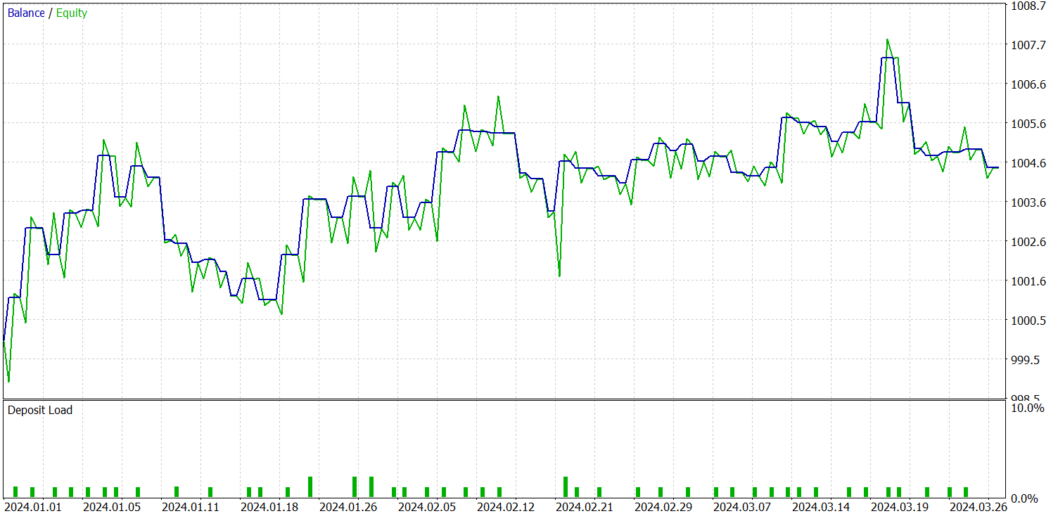
At first glance, comparing the test results between the current and baseline models yields mixed impressions. On one hand, we observe a decline in the profit factor from 1.4 to 1.29. On the other hand, thanks to a 2.5x increase in the number of trades, the total profit for the same test period grew proportionally.

In addition, unlike the baseline model, the new model shows a consistent upward balance trend throughout the test period. However, only short positions were executed. This may be due to a stronger focus on global trends in the smoothed values. As a result, some local trends may be ignored during noise filtering.

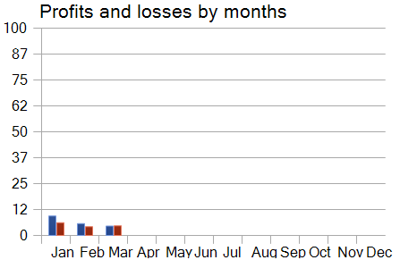
Nevertheless, when analyzing the model's monthly performance curve, we observe a gradual decrease in profitability over time. This observation supports the hypothesis we made in the previous article: the representativeness of the training dataset diminishes as the test period lengthens.

Conclusion

In this article, we explored the NAFS (Node-Adaptive Feature Smoothing) method, which is a simple yet effective non-parametric approach for constructing node representations in graphs without requiring parameter training. It combines smoothed neighbor features, and by using ensembles of different smoothing strategies, produces robust and informative final embeddings.

On the practical side, we implemented our interpretation of the proposed methods in MQL5, trained the constructed models on real historical data, and tested them on out-of-sample datasets. Based on our experiments, we can conclude that the proposed approaches demonstrate potential. They can be combined with other frameworks. Also, their integration can improve the efficiency of baseline models.

References

• NAFS: A Simple yet Tough-to-beat Baseline for Graph Representation Learning
• Other articles from this series

Programs used in the article

#	Name	Type	Description
1	Research.mq5	Expert Advisor	EA for collecting examples
2	ResearchRealORL.mq5	Expert Advisor	EA for collecting examples using the Real-ORL method
3	Study.mq5	Expert Advisor	Model training EA
4	Test.mq5	Expert Advisor	Model testing EA
5	Trajectory.mqh	Class library	System state description structure
6	NeuroNet.mqh	Class library	A library of classes for creating a neural network
7	NeuroNet.cl	Library	OpenCL program code library