
Neural networks made easy (Part 16): Practical use of clustering

Contents
- Introduction
- 1. Theoretical aspects of the utilization of clustering results
- 2. Using clustering as an independent solution
- 3. Using clustering results as input
- Conclusion
- List of references
- Programs used in the article
Introduction
The previous two articles were devoted to data clustering. But our main goal is to learn how to use all the considered methods to solve specific practical problems. In particular, trading related cases. When we started considering unsupervised learning methods, we talked about the possibility of using the results obtained both independently and as input data for other models. In this article, we will consider possible use cases for clustering results.
1. Theoretical aspects of the utilization of clustering results
Before we move on to the practical implementation of examples related to the use of clustering results, let us talk a little about the theoretical aspects of these approaches.
The first option for using data clustering results is to try to get the most out of them for practical use without any additional funds. I.e., the clustering results can be used independently, to make trading decisions. I would like to remind that unsupervised learning methods are not used for solving regression tasks. While forecasting the nearest price movement is precisely a regression task. At first glance, we see some kind of conflict.
But look from the other side. Considering the theoretical aspects of clustering, we have already compared clustering with the definition of graphic patterns. Like with chart patterns, we can collect statistics on the price behavior after an element of a particular cluster appears on the chart. Well, that will not give us a causal relationship. But such relationship does not exist in any mathematical model built using neural networks. We only build probabilistic models without diving deep into causal relationships.
To collect statistics, we need an already trained clustering model and labeled data. Since our clustering model has already been trained, the labeled data set can be much smaller than the training sample. However, it should be sufficient and representative.
At first glance, this approach may resemble supervised learning. But it has two major differences:
- The labeled sample size can be smaller as there is no risk of overfitting.
- In supervised learning, we use an iterative process during which optimal weight coefficients are selected. This requires several training epochs with high resource and time costs. The first pass is enough to collect statistics. No model adjustment is performed in this case.
I hope the idea is simple. We will consider the implementation of such a model a bit later.
The disadvantage of this option is that the distance to the center of the cluster is ignored. In other words, we will have the same result for elements close to the cluster center ("an ideal pattern") and elements on the borders of the cluster. You can try to increase the number of clusters in an effort to reduce the maximum distance of elements from the center. But the effectiveness of this approach will be minimal, provided that we have correctly chosen the number of clusters according to the loss function graph.
You can try to solve this issue using the second application of clustering results: as the source data of another model. But note that by inputting the cluster number in the form of a number or a vector into the second model, we will receive at most data comparable to the results of the statistical method considered above. Spending additional costs to receive the same result makes no sense.
Instead of the cluster number, we can input the distance to cluster centers into the model. We should not forget that neural networks prefer normalized data. We normalize the data of the distances vector using the Softmax function.
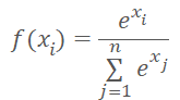
But Softmax is based on the exponent, the graph of which is shown in the figure below.

Now let us think about which vector we will get as a result of normalizing the distances to the centers of clusters with the Softmax function. It is obvious that all distances are positive. The greater the distance, the greater the exponent and the more the function value changes with the same change in its argument. Therefore, the maximum distances will receive larger weight. As the distance decreases, the differences between the values decrease. Thus, by using this simple normalization we will get a vector describing to which clusters the element does not belong, thus making it more difficult to determine the cluster to which the element belongs. We need the opposite.
It would seem that the situation could be corrected by simply changing the sign of the distance value. But in the area of negative arguments, the value of the exponential function approaches 0. As the argument decreases, the deviation of the function values also tends to 0.
As a solution to the above problems, we can first normalize the distances in the range from 0 to 1. And then apply the Softmax function to "1—X".
The choice of the model to which normalized values are input depends on the problem and is beyond the scope of this article.
Now that we have discussed the main theoretical approaches to the use of clustering results, we can move on to the practical part of our article.
2. Using clustering as an independent solution
We will start the implementation of the statistical method by writing the code of another kernel KmeansStatistic in the OpenCL program (file unsupervised.cl), which will calculate the statistics related to each cluster signal processing. The way this process is organized ma resemble supervised learning. In fact, we do need labeled data. But there is a fundamental difference between this process and the previously backpropagation method. Previously, we optimized the model function to obtain results very close to reference values. Now we will not change the model in any way. Instead, we will collect statistics of the system's reaction to the appearance of a particular pattern.
We will pass in parameters to the kernel pointers to three data buffers and the total number of elements in the training set. But we will not pass the training sample in this kernel parameters. To execute this functionality, we do not need to know the contents of the system state description vector. At this stage, it is enough for us to know to which class the analyzed system state belongs. Therefore, instead of passing the training sample in the kernel parameters, we will pass a pointer to the clusters vector, which contains cluster identifiers for each system state from the training set.
The second input data buffer target will contain a tensor describing the reaction of the system after the appearance of a particular buffer. This tensor will have three logical flags to describe the signal after the pattern appears: buy, sell, undefined. Through the use of flags, the calculation of signal statistics becomes easier and more intuitive. However, at the same time, it limits the variability of possible signals. Therefore, the use of this method must comply with the technical requirements of the task. In this series of articles, we evaluated all considered algorithms in terms of their ability to identify fractal formation before the formation of the last candlestick begins. As you know, we need three candlesticks to determine a fractal on a chart. Therefore, in fact, we can only determine it after the formation of the third candlestick of the pattern. However, we want to find a way to determine the formation of a pattern when only two candlesticks of the future pattern are formed. Of course, with some degree of probability. To solve this problem, it is enough to use target signals of three flags for each pattern.
Also, various training samples can be used to collect signal statistics after patterns appear and to train the model. For example, the model can be trained over a sufficiently long historical interval so that the model can learn the features of the state of the analyzed system as much as possible. While a shorter historical period can be used to label the data and to collect statistics. Of course, before collecting statistics, we been to cluster the corresponding clusters. Because to ensure correct statistics collection, the data must be comparable.
Let us get back to our algorithm. Kernel execution will run in a one-dimensional task space. The number of parallel threads will be equal to the number of clusters created.
At the beginning of the kernel, we define the ID of the current thread which determines the sequence number of the analyzed cluster. Also, we immediately determine the shift in the tensor of probabilistic results. Prepare private variables to count the number of occurrences of each signal: buy, sell, skip. Assign the initial value of 0 to each variable.
Next, implement a loop with the number of iterations equal to the number of elements in the training sample. In the loop body, first check whether the system state belongs to the analyzed cluster. If it belongs, add the contents of the target flags tensor to the relevant private variables.
For target values we use the flags that can only be 0 or 1. We will use mutually exclusive signals. This means that at a moment of time it is possible to have 1 in only one flag for each individual state of the system. Thanks to this property, we do not have to use a separate counter for the number of pattern occurrences. Instead, after exiting the loop, we sum up all three private variables to get the total number of pattern occurrences.
Now we need to translate the natural sums of signals into the field of probabilistic mathematics. To do this, we divide the value of each private variable by the total number of pattern occurrences. However, there are a few moments to pay attention to. First, it is necessary to eliminate the possibility of a critical divide-by-zero error. Second, we need real probabilities that we can trust. Let me explain that. For example, if a certain parameter occurs once, the probability of such a signal will be 100%. But can such a signal be trusted? Of course not. Most likely, its appearance is accidental. Therefore, for all patterns that occurred less than 10 times, all signals will be assigned zero probabilities.
__kernel void KmeansStatistic(__global double *clusters,
                              __global double *target,
                              __global double *probability,
                              int total_m
                             )
  {
   int c = get_global_id(0);
   int shift_c = c * 3;
   double buy = 0;
   double sell = 0;
   double skip = 0;
   for(int i = 0; i < total_m; i++)
     {
      if(clusters[i] != c)
         continue;
      int shift = i * 3;
      buy += target[shift];
      sell += target[shift + 1];
      skip += target[shift + 2];
     }
//---
   int total = buy + sell + skip;
   if(total < 10)
     {
      probability[shift_c] = 0;
      probability[shift_c + 1] = 0;
      probability[shift_c + 2] = 0;
     }
   else
     {
      probability[shift_c] = buy / total;
      probability[shift_c + 1] = sell / total;
      probability[shift_c + 2] = skip / total;
     }
  }
After creating a kernel in the OpenCL program, we proceed to working on the side of the main program. First, we add constants for working with the earlier created kernel. Of course, the naming of constants must comply with our naming policy.
#define def_k_kmeans_statistic   4
#define def_k_kms_clusters       0
#define def_k_kms_targers        1
#define def_k_kms_probability    2
#define def_k_kms_total_m        3
After creating the constants, move on to the OpenCLCreate function in which we change the total number of used kernels. We will also add the creation of a new kernel.
COpenCLMy *OpenCLCreate(string programm)
  {
   ...............
//---
   if(!result.SetKernelsCount(5))
     {
      delete result;
      .return NULL;
     }
//---
   ...............
//---
   if(!result.KernelCreate(def_k_kmeans_statistic, "KmeansStatistic"))
     {
      delete result;
      .return NULL;
     }
//---
   return result;
  }
Now we need to implement the call of this kernel on the side of the main program.
To enable this call, let us create the Statistic method in our CKmeans class. The new method will receive in parameters pointers to two data buffers: a training sample and reference values. Although the data set resembles supervised learning, there is a fundamental difference in the approaches. During supervised learning, we optimized the model to obtain optimal results, which is an iterative process. Now we simply collect statistics in one pass.
In the method body, we check the relevance of the pointer to the target values buffer and call the training sample clustering method. Do not forget that the training sample in this case can differ from the one used to train the model, but it must correspond to the target values.
bool CKmeans::Statistic(CBufferDouble *data, CBufferDouble *targets)
  {
   if(CheckPointer(targets) == POINTER_INVALID ||
      !Clustering(data))
      return false;
Next, we initialize the buffer to write the probabilistic values of the predicted system behavior. I deliberately do not use the expression "response to pattern" since we are not analyzing causality. It can be direct or indirect. There can be no relation at all. We only collect statistics using historical data.
   if(CheckPointer(c_aProbability) == POINTER_INVALID)
     {
      c_aProbability = new CBufferDouble();
      if(CheckPointer(c_aProbability) == POINTER_INVALID)
         return false;
     }
   if(!c_aProbability.BufferInit(3 * m_iClusters, 0))
      return false;
//---
   int total = c_aClasters.Total();
   if(!targets.BufferCreate(c_OpenCL) ||
      !c_aProbability.BufferCreate(c_OpenCL))
      return false;
After creating a buffer, we load the required data to the OpenCL context memory and implement the kernel call procedure. We first pass the kernel parameters, determine the dimension of the task space and offsets in each dimension. After that, we place the kernel in the execution queue and read the result of the operations. During the execution of operations, be sure to control the process at each step.
   if(!c_OpenCL.SetArgumentBuffer(def_k_kmeans_statistic, def_k_kms_probability, c_aProbability.GetIndex()))
      return false;
   if(!c_OpenCL.SetArgumentBuffer(def_k_kmeans_statistic, def_k_kms_targers, targets.GetIndex()))
      return false;
   if(!c_OpenCL.SetArgumentBuffer(def_k_kmeans_statistic, def_k_kms_clusters, c_aClasters.GetIndex()))
      return false;
   if(!c_OpenCL.SetArgument(def_k_kmeans_statistic, def_k_kms_total_m, total))
      return false;
   uint global_work_offset[1] = {0};
   uint global_work_size[1];
   global_work_size[0] = m_iClusters;
   if(!c_OpenCL.Execute(def_k_kmeans_statistic, 1, global_work_offset, global_work_size))
      return false;
   if(!c_aProbability.BufferRead())
      return false;
//---
   data.BufferFree();
   targets.BufferFree();
//---
   return true;
  }
If the kernel is successfully executed, in the c_aProbability buffer we will receive the probabilities of the occurrence of each pattern. We only need to clear the memory and complete the method.
But the considered procedure can be attributed to model training. For practical use, we need to obtain the real-time system behavior probabilities. For this purpose, we create another method GetProbability. In the method parameters we will only pass a sample for clustering. It is very important to have the c_aProbability probability matrix formed before calling the method. Therefore, this is the first thing we check in the method body. After that start clustering the received data. Again, check the operation execution result.
CBufferDouble *CKmeans::GetProbability(CBufferDouble *data)
  {
   if(CheckPointer(c_aProbability) == POINTER_INVALID ||
      !Clustering(data))
      .return NULL;
The specific feature of this method is that as a result of its operation, we return not a boolean value but a pointer to the data buffer. Therefore, in the next step we create a new buffer to collect data.
   CBufferDouble *result = new CBufferDouble();
   if(CheckPointer(result) == POINTER_INVALID)
      return result;
We assume that in real time we will receive probabilistic data for a small number of records. Most often there will be only one record — the current state of the system. Therefore, we will not take further work to parallel computing. We will implement a loop to iterate over the buffer of identifiers of the studied data clusters. In the loop body, we transfer the probabilities of the corresponding clusters to the result buffer.
   int total = c_aClasters.Total();
   if(!result.Reserve(total * 3))
     {
      delete result;
      return result;
     }
   for(int i = 0; i < total; i++)
     {
      int k = (int)c_aClasters.At(i) * 3;
      if(!result.Add(c_aProbability.At(k)) ||
         !result.Add(c_aProbability.At(k + 1)) ||
         !result.Add(c_aProbability.At(k + 2))
        )
        {
         delete result;
         return result;
        }
     }
//---
   return result;
  }
Note that in the results buffer the probabilities will be arranged in the same sequence as the system states in the analyzed sample. If the sample contained data belonging to one cluster, the system behavior probabilities will be repeated.
To test the method, we have created the "kmeans_stat.mq5" Expert Advisor. Its code is available in the attachment. As can be understood from the file name, it provides statistics on the probabilities of the appearance of fractals after each pattern.
We conducted the experiment using the 500-cluster model which was trained in the previous article. The results are shown in the screenshot below.

The provided data prove that the use of this approach makes it possible to predict the market reaction after fractal appearance with a probability of 30-45%. This is quite a good result. Especially considering the fact that we did not use multilayer neural networks.
3. Using clustering results as input
Let us move on to the implementation of the second variant of using clustering results. In this approach, we are going to input clustering results of clustering into another model. Actually, this can be any model of your choice suitable for your problem, including a neural network using supervised learning algorithms.
We have previously determined that when implementing this approach, clustering results will be presented as a normalized vector of distances to the centers of clusters. To implement this functionality, we need to create another kernel KmeansSoftMax in OpenCL program unsupervised.cl.
We will not recalculate the distances to the center of each cluster in the new kernel, because this function is already executed in the KmeansCulcDistance kernel. In KmeansSoftMax, we will only normalize available data.
In the kernel parameters, we will pass pointers to two data buffers and the total number of clusters used. Among data buffers there will be one source data buffer distance and one results buffer softmax. Both buffers have the same sizes and are vector representations of a matrix, the rows of which represent individual elements of the sequence, and the columns represent clusters.
The kernel will be launched in a one-dimensional task space according to the number of elements in the clustered sample. I deliberately do not refer to it as a "training sample", because the kernel can be used both when training the second model and in resulting operation. It is obvious that the data input in these two variants will be different.
Before we proceed to the implementation of the kernel code, let us remember that we have slightly changed the normalization functions and it is now as follows.
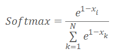
where x is the distance to the cluster center normalized in the range between 0 and 1.
Now let us look at the implementation of the above formula. In the kernel body, we first determine the thread identifier, which indicates the analyzed element of the sequence. We also determine the shift in buffers up to the beginning of the analyzed vector. Since the initial data and results tensors are of the same size, The offset in the two buffers will also be the same.
Next, to normalize distances in the range between 0 and 1, we need to find the maximum deviation from the cluster center. Remember that when calculating distances, we used squared deviations. It means that all values in the distance vector will be positive. This makes things a little easier. We declare the private variable m to write the maximum distance and initialize it with the value of the first element of our vector. Next, we create a loop that iterates through all the elements of the vector. In the vector body, we will compare the values of elements with the saved value and write the maximum value into the variable.
Once the highest value is determined, we can move on to calculating exponential values for each element. Also, we can immediately calculate the sum of exponential values of the entire vector. To find the sum, we initialize the private variable sum with the 0 value. The relevant arithmetical operations will be performed in the next loop. The number of loop iterations is equal to the number of clusters in the model. In the loop body, we first save in a private variable the exponential value of the normalized and "inverted" distance to the cluster center. Add the resulting value to the sum and then move to the results buffer. The use of a private variable before writing values to the buffer minimizes the number of slow global memory accesses.
Once the loop iterations are completed, we need to normalize the data by dividing the obtained exponential values by the total sum. To execute these operations, let us create another loop with the number of iterations equal to the number of clusters. Exit the kernel after the loop is completed.
__kernel void KmeansSoftMax(__global double *distance,
                            __global double *softmax,
                            inсt total_k
                           )
  {
   int i = get_global_id(0);
   int shift = i * total_k;
   double m=distance[shift];
   for(int k = 1; k < total_k; k++)
      m =  max(distance[shift + k],m);
   double sum = 0;
   for(int k = 0; k < total_k; k++)
     {
      double value =  exp(1-distance[shift + k]/m);
      sum += value;
      softmax[shift + k] = value;
     }
   for(int k = 0; k < total_k; k++)
      softmax[shift + k] /= sum;
  }
We have expanded the functionality of the OpenCL program. Now we only need to add the kernel call from our CKmeans class. We will stick to the same scheme that we used above to add the previous kernel call code.
First, add constants according to the naming policy.
#define def_k_kmeans_softmax     5
#define def_k_kmsm_distance      0
#define def_k_kmsm_softmax       1
#define def_k_kmsm_total_k       2
Then, we add the kernel declaration in the OpenCL context initialization function OpenCLCreate.
COpenCLMy *OpenCLCreate(string programm)
  {
   ...............
//---
   if(!result.SetKernelsCount(6))
     {
      delete result;
      .return NULL;
     }
//---
   ...............
//---
   if(!result.KernelCreate(def_k_kmeans_softmax, "KmeansSoftMax"))
     {
      delete result;
      .return NULL;
     }
//---
   return result;
  }
And of course, we need a new method of our class CKmeans::SoftMax. The method receives in parameters a pointer to the initial data buffer. As a result of operation, the method will return a result buffer of the same size.
In the method body, we first check whether our clustering class was previously trained. If necessary, initialize the model training process. Iwould like to remind here that we set a limitation on the maximum size of the learning sample in the model training method. Therefore, id the model has not been previously trained, a big enough sample should be passed in the parameters to the method. Otherwise, the method will return an invalid pointer to the results buffer. If the data clustering model has already been trained, then the restriction on the sample size is lifted.
CBufferDouble *CKmeans::SoftMax(CBufferDouble *data)
  {
   if(!m_bTrained && !Study(data, (c_aMeans.Maximum() == 0)))
      .return NULL;
In the next step, we check the validity of the pointers to the used objects. It may seem strange that we first call the learning method and then check object pointers. In fact, the learning method itself has a similar block of controls. If we always called the model training method before continuing operations, these controls would be unnecessary as they repeat controls inside the training method. But if we use a pretrained model, we will not call the training method and hence we will not have its controls. While further execution of operations with invalid pointers will lead to critical errors. Therefore, we have to re-check the pointers.
   if(CheckPointer(data) == POINTER_INVALID || CheckPointer(c_OpenCL) == POINTER_INVALID)
      .return NULL;
After checking the pointers, let us check the size of the source data buffer. It must contain at least the vector with the description of the 1st state of the system. Also, the amount of data in the buffer must be a multiple of the system state description vector.
   int total = data.Total();
   if(total <= 0 || m_iClusters < 2 || (total % m_iVectorSize) != 0)
      .return NULL;
Then we will determine the number of system states that should be distributed among clusters.
   int rows = total / m_iVectorSize;
   if(rows < 1)
      .return NULL;
Next, we need to initialize buffers for calculating and normalizing distances. The initialization algorithm is quite simple. We first check the validity of the buffer pointer and, if necessary, create a new object. Then we fill the buffer with zero values.
   if(CheckPointer(c_aDistance) == POINTER_INVALID)
     {
      c_aDistance = new CBufferDouble();
      if(CheckPointer(c_aDistance) == POINTER_INVALID)
         .return NULL;
     }
   c_aDistance.BufferFree();
   if(!c_aDistance.BufferInit(rows * m_iClusters, 0))
      .return NULL;

   if(CheckPointer(c_aSoftMax) == POINTER_INVALID)
     {
      c_aSoftMax = new CBufferDouble();
      if(CheckPointer(c_aSoftMax) == POINTER_INVALID)
         .return NULL;
     }
   c_aSoftMax.BufferFree();
   if(!c_aSoftMax.BufferInit(rows * m_iClusters, 0))
      .return NULL;
To complete the preparatory work, we create the necessary data buffers in the OpenCL context.
   if(!data.BufferCreate(c_OpenCL) ||
      !c_aMeans.BufferCreate(c_OpenCL) ||
      !c_aDistance.BufferCreate(c_OpenCL) ||
      !c_aSoftMax.BufferCreate(c_OpenCL))
      .return NULL;
This completes the preparatory work. Now we move on to calling the necessary kernels. To implement the full functionality of the method, we need to create a sequential call of two kernels:
- determining distances to cluster centers KmeansCulcDistance;
- normalization of distances KmeansSoftMax.
The kernel call algorithm is quite simple and is similar to that used in the previously described method of statistical use of clustering results. First, we need to pass parameters to the kernel.
   if(!c_OpenCL.SetArgumentBuffer(def_k_kmeans_distance, def_k_kmd_data, data.GetIndex()))
      .return NULL;
   if(!c_OpenCL.SetArgumentBuffer(def_k_kmeans_distance, def_k_kmd_means, c_aMeans.GetIndex()))
      .return NULL;
   if(!c_OpenCL.SetArgumentBuffer(def_k_kmeans_distance, def_k_kmd_distance, c_aDistance.GetIndex()))
      .return NULL;
   if(!c_OpenCL.SetArgument(def_k_kmeans_distance, def_k_kmd_vector_size, m_iVectorSize))
      .return NULL;
Then we specify the dimension of the problem space and the offset in each dimension.
   uint global_work_offset[2] = {0, 0};
   uint global_work_size[2];
   global_work_size[0] = rows;
   global_work_size[1] = m_iClusters;
Then we put the kernel in the execution queue and read the operation execution results.
   if(!c_OpenCL.Execute(def_k_kmeans_distance, 2, global_work_offset, global_work_size))
      .return NULL;
   if(!c_aDistance.BufferRead())
      .return NULL;
Repeat the operations for the second kernel.
   if(!c_OpenCL.SetArgumentBuffer(def_k_kmeans_softmax, def_k_kmsm_distance, c_aDistance.GetIndex()))
      .return NULL;
   if(!c_OpenCL.SetArgumentBuffer(def_k_kmeans_softmax, def_k_kmsm_softmax, c_aSoftMax.GetIndex()))
      .return NULL;
   if(!c_OpenCL.SetArgument(def_k_kmeans_softmax, def_k_kmsm_total_k, m_iClusters))
      .return NULL;
   uint global_work_offset1[1] = {0};
   uint global_work_size1[1];
   global_work_size1[0] = rows;
   if(!c_OpenCL.Execute(def_k_kmeans_softmax, 1, global_work_offset1, global_work_size1))
      .return NULL;
   if(!c_aSoftMax.BufferRead())
      .return NULL;
In the end, clear the memory of the OpenCL context and exit the method, while returning a pointer to the result buffer.
   data.BufferFree();
   c_aDistance.BufferFree();
//---
   return c_aSoftMax;
  }
This completes operations related to modification in our k-means clustering class CKmeans. Now we can move on to testing the approach. For this purpose, let us create an Expert Advisor entitled kmeans_net.mq5, which is modeled after Expert Advisors from articles about supervised learning algorithms. To test the implementation, I input the clustering results into a fully-connected perceptron with three hidden layers. The full Expert Advisor code is available in the attachment. Pay attention to the Train learning function.
At the function beginning, we initialize an object instance to work with the OpenCL context within the clustering class. Then we pass the pointer to the created object to our clustering class. Do not forget to check the operation execution results.
void Train(datetime StartTrainBar = 0)
  {
   COpenCLMy *opencl = OpenCLCreate(cl_unsupervised);
   if(CheckPointer(opencl) == POINTER_INVALID)
     {
      ExpertRemove();
      return;
     }
   if(!Kmeans.SetOpenCL(opencl))
     {
      delete opencl;
      ExpertRemove();
      return;
     }
After successful initialization of objects, we determine the boundaries of the training period.
   MqlDateTime start_time;
   TimeCurrent(start_time);
   start_time.year -= StudyPeriod;
   if(start_time.year <= 0)
      start_time.year = 1900;
   datetime st_time = StructToTime(start_time);
Loading historical data. Please note that indicator data loaded into buffers is represented by timeseries, unlike quotes. This is important, since we get the reverse sorting of elements in arrays. Therefore, to enable data comparability, we must invert the array of quotes into a timeseries.
   int bars = CopyRates(Symb.Name(), TimeFrame, st_time, TimeCurrent(), Rates);
   if(!RSI.BufferResize(bars) || !CCI.BufferResize(bars) || !ATR.BufferResize(bars) || !MACD.BufferResize(bars))
     {
      ExpertRemove();
      return;
     }
   if(!ArraySetAsSeries(Rates, true))
     {
      ExpertRemove();
      return;
     }

   RSI.Refresh();
   CCI.Refresh();
   ATR.Refresh();
   MACD.Refresh();
After successfully loading the historical data, load the pretrained clustering model.
   int handl = FileOpen(StringFormat("kmeans_%d.net", Clusters), FILE_READ | FILE_BIN);
   if(handl == INVALID_HANDLE)
     {
      ExpertRemove();
      return;
     }
   if(FileReadInteger(handl) != Kmeans.Type())
     {
      ExpertRemove();
      return;
     }
   bool result = Kmeans.Load(handl);
   FileClose(handl);
   if(!result)
     {
      ExpertRemove();
      return;
     }
Proceed to forming a training sample and target values.
   int total = bars - (int)HistoryBars - 1;
   double data[], fractals[];
   if(ArrayResize(data, total * 8 * HistoryBars) <= 0 ||
      ArrayResize(fractals, total * 3) <= 0)
     {
      ExpertRemove();
      return;
     }
//---
   for(int i = 0; (i < total && !IsStopped()); i++)
     {
      Comment(StringFormat("Create data: %d of %d", i, total));
      for(int b = 0; b < (int)HistoryBars; b++)
        {
         int bar = i + b;
         int shift = (i * (int)HistoryBars + b) * 8;
         double open = Rates[bar].open;
         data[shift] = open - Rates[bar].low;
         data[shift + 1] = Rates[bar].high - open;
         data[shift + 2] = Rates[bar].close - open;
         data[shift + 3] = RSI.GetData(MAIN_LINE, bar);
         data[shift + 4] = CCI.GetData(MAIN_LINE, bar);
         data[shift + 5] = ATR.GetData(MAIN_LINE, bar);
         data[shift + 6] = MACD.GetData(MAIN_LINE, bar);
         data[shift + 7] = MACD.GetData(SIGNAL_LINE, bar);
        }
      int shift = i * 3;
      int bar = i + 1;
      fractals[shift] = (int)(Rates[bar - 1].high <= Rates[bar].high && Rates[bar + 1].high < Rates[bar].high);
      fractals[shift + 1] = (int)(Rates[bar - 1].low >= Rates[bar].low && Rates[bar + 1].low > Rates[bar].low);
      fractals[shift + 2] = (int)((fractals[shift] + fractals[shift]) == 0);
     }
   if(IsStopped())
     {
      ExpertRemove();
      return;
     }
   CBufferDouble *Data = new CBufferDouble();
   if(CheckPointer(Data) == POINTER_INVALID ||
      !Data.AssignArray(data))
      return;
   CBufferDouble *Fractals = new CBufferDouble();
   if(CheckPointer(Fractals) == POINTER_INVALID ||
      !Fractals.AssignArray(fractals))
      return;
Since our clustering methods can work with initial data arrays, we can cluster the entire training sample at once.
   ResetLastError();
   CBufferDouble *softmax = Kmeans.SoftMax(Data);
   if(CheckPointer(softmax) == POINTER_INVALID)
     {
      printf("Runtime error %d", GetLastError());
      ExpertRemove();
      return;
     }
After successful completion of all these operations, the softmax buffer will contain a training sample for our perceptron. We have also prepared target values in advance. So, we can move on to the second model training cycle.
Similar to supervised learning algorithm testing, the model training will be implemented using two nested loops. The outer loop will count training epoch. We exit the loop upon a certain event.
First, we will do a little preparatory work. We need to initialize the necessary local variables.
  if(CheckPointer(TempData) == POINTER_INVALID)
     {
      TempData = new CArrayDouble();
      if(CheckPointer(TempData) == POINTER_INVALID)
        {
         ExpertRemove();
         return;
        }
     }
   delete opencl;
   double prev_un, prev_for, prev_er;
   dUndefine = 0;
   dForecast = 0;
   dError = -1;
   dPrevSignal = 0;
   bool stop = false;
   int count = 0;
   do
     {
      prev_un = dUndefine;
      prev_for = dForecast;
      prev_er = dError;
      ENUM_SIGNAL bar = Undefine;
      //---
      stop = IsStopped();
And only then we will move on to the nested loop. The number of nested loop iterations will be equal to the size of the training sample minus a small "tail" of the validation zone.
Even though the number of iterations is equal to the sample size, we will every time select a random element for the learning process. We will define it at the beginning of the nested loop. The use of random vectors from a training sample ensures uniform model training.
      for(int it = 0; (it < total - 300 && !IsStopped()); it++)
        {
         int i = (int)((MathRand() * MathRand() / MathPow(32767, 2)) * (total - 300)) + 300;
By the index of a randomly selected element, determine the offset in the initial data buffer and copy the necessary vector to the temporary buffer.
         TempData.Clear();
         int shift = i * Clusters;
         if(!TempData.Reserve(Clusters))
           {
            if(CheckPointer(Data) == POINTER_DYNAMIC)
               delete Data;
            if(CheckPointer(Fractals) == POINTER_DYNAMIC)
               delete Fractals;
            if(CheckPointer(softmax) == POINTER_DYNAMIC)
               delete softmax;
            if(CheckPointer(opencl) == POINTER_DYNAMIC)
               delete opencl;
            Comment("");
            //---
            ExpertRemove();
            return;
           }
         for(int c = 0; c < Clusters; c++)
            if(!TempData.Add(softmax.At(shift + c)))
              {
               if(CheckPointer(Data) == POINTER_DYNAMIC)
                  delete Data;
               if(CheckPointer(Fractals) == POINTER_DYNAMIC)
                  delete Fractals;
               if(CheckPointer(softmax) == POINTER_DYNAMIC)
                  delete softmax;
               if(CheckPointer(opencl) == POINTER_DYNAMIC)
                  delete opencl;
               Comment("");
               //---
               ExpertRemove();
               return;
              }
After generating the initial data vector, we input it into the forward method of our neural network. After a successful forward pass, we get its result.
         if(!Net.feedForward(TempData))
           {
            if(CheckPointer(Data) == POINTER_DYNAMIC)
               delete Data;
            if(CheckPointer(Fractals) == POINTER_DYNAMIC)
               delete Fractals;
            if(CheckPointer(softmax) == POINTER_DYNAMIC)
               delete softmax;
            if(CheckPointer(opencl) == POINTER_DYNAMIC)
               delete opencl;
            Comment("");
            //---
            ExpertRemove();
            return;
           }
         Net.getResults(TempData);
Normalize the results using the Softmax function.
         double sum = 0;
         for(int res = 0; res < 3; res++)
           {
            double temp = exp(TempData.At(res));
            sum += temp;
            TempData.Update(res, temp);
           }
         for(int res = 0; (res < 3 && sum > 0); res++)
            TempData.Update(res, TempData.At(res) / sum);
To visually track the model learning process, let us display the current state on the chart.
         switch(TempData.Maximum(0, 3))
           {
            case 1:
               dPrevSignal = (TempData[1] != TempData[2] ? TempData[1] : 0);
               break;
            case 2:
               dPrevSignal = -TempData[2];
               break;
            default:
               dPrevSignal = 0;
               break;
           }
         string s = StringFormat("Study -> Era %d -> %.2f -> Undefine %.2f%% foracast %.2f%%\n %d of %d -> %.2f%%
                                 \nError %.2f\n%s -> %.2f ->> Buy %.5f - Sell %.5f - Undef %.5f",
                                 count, dError, dUndefine, dForecast, it + 1, total - 300,
                                 (double)(it + 1.0) / (total - 300) * 100, Net.getRecentAverageError(),
                                 EnumToString(DoubleToSignal(dPrevSignal)), dPrevSignal, TempData[1], TempData[2],
                                 TempData[0]);
         Comment(s);
         stop = IsStopped();
At the end of the loop iteration, call the back propagation method and update the wight matrix in our model.
         if(!stop)
           {
            shift = i * 3;
            TempData.Clear();
            TempData.Add(Fractals.At(shift + 2));
            TempData.Add(Fractals.At(shift));
            TempData.Add(Fractals.At(shift + 1));
            Net.backProp(TempData);
            ENUM_SIGNAL signal = DoubleToSignal(dPrevSignal);
            if(signal != Undefine)
              {
               if((signal == Sell && Fractals.At(shift + 1) == 1) || (signal == Buy && Fractals.At(shift) == 1))
                  dForecast += (100 - dForecast) / Net.recentAverageSmoothingFactor;
               else
                  dForecast -= dForecast / Net.recentAverageSmoothingFactor;
               dUndefine -= dUndefine / Net.recentAverageSmoothingFactor;
              }
            else
              {
               if(Fractals.At(shift + 2) == 1)
                  dUndefine += (100 - dUndefine) / Net.recentAverageSmoothingFactor;
              }
           }
        }
After each training epoch, we will display graphic labels on the validation plot. To implement this functionality, let us create another nested loop. Operations in the loop body mostly repeat the earlier described loop, with only two main differences:
- We will take elements in the order they are, instead of random selection.
- No back propagation method will be performed here.
In the validation sample, check how the model works on new data without overfitting the parameter. That is why there is no back propagation method. Therefore, the model operation result does not depend on data feeding sequence (an exception for recurrent models). Thus, we do not spend resources to generate a random number and take all the states of the system sequentially.
      count++;
      for(int i = 0; i < 300; i++)
        {
         TempData.Clear();
         int shift = i * Clusters;
         if(!TempData.Reserve(Clusters))
           {
            if(CheckPointer(Data) == POINTER_DYNAMIC)
               delete Data;
            if(CheckPointer(Fractals) == POINTER_DYNAMIC)
               delete Fractals;
            if(CheckPointer(softmax) == POINTER_DYNAMIC)
               delete softmax;
            if(CheckPointer(opencl) == POINTER_DYNAMIC)
               delete opencl;
            Comment("");
            //---
            ExpertRemove();
            return;
           }

         for(int c = 0; c < Clusters; c++)
            if(!TempData.Add(softmax.At(shift + c)))
              {
               if(CheckPointer(Data) == POINTER_DYNAMIC)
                  delete Data;
               if(CheckPointer(Fractals) == POINTER_DYNAMIC)
                  delete Fractals;
               if(CheckPointer(softmax) == POINTER_DYNAMIC)
                  delete softmax;
               if(CheckPointer(opencl) == POINTER_DYNAMIC)
                  delete opencl;
               Comment("");
               //---
               ExpertRemove();
               return;
              }
         if(!Net.feedForward(TempData))
           {
            if(CheckPointer(Data) == POINTER_DYNAMIC)
               delete Data;
            if(CheckPointer(Fractals) == POINTER_DYNAMIC)
               delete Fractals;
            if(CheckPointer(softmax) == POINTER_DYNAMIC)
               delete softmax;
            if(CheckPointer(opencl) == POINTER_DYNAMIC)
               delete opencl;
            Comment("");
            //---
            ExpertRemove();
            return;
           }
         Net.getResults(TempData);

         double sum = 0;
         for(int res = 0; res < 3; res++)
           {
            double temp = exp(TempData.At(res));
            sum += temp;
            TempData.Update(res, temp);
           }
         for(int res = 0; (res < 3 && sum > 0); res++)
            TempData.Update(res, TempData.At(res) / sum);
         //---
         switch(TempData.Maximum(0, 3))
           {
            case 1:
               dPrevSignal = (TempData[1] != TempData[2] ? TempData[1] : 0);
               break;
            case 2:
               dPrevSignal = -TempData[2];
               break;
            default:
               dPrevSignal = 0;
               break;
           }
Add the display of objects on the chart and exit the validation cycle.
         if(DoubleToSignal(dPrevSignal) == Undefine)
            DeleteObject(Rates[i + 2].time);
         else
            DrawObject(Rates[i + 2].time, dPrevSignal, Rates[i + 2].high, Rates[i + 2].low);
        }
Before completing the iteration of the outer loop, we save the current model state and add the error value to the training dynamics file.
      if(!stop)
        {
         dError = Net.getRecentAverageError();
         Net.Save(FileName + ".nnw", dError, dUndefine, dForecast, Rates[0].time, false);
         printf("Era %d -> error %.2f %% forecast %.2f", count, dError, dForecast);
         ChartScreenShot(0, FileName + IntegerToString(count) + ".png", 750, 400);
         int h = FileOpen(FileName + ".csv", FILE_READ | FILE_WRITE | FILE_CSV);
         if(h != INVALID_HANDLE)
           {
            FileSeek(h, 0, SEEK_END);
            FileWrite(h, eta, count, dError, dUndefine, dForecast);
            FileFlush(h);
            FileClose(h);
           }
        }
     }
   while((!(DoubleToSignal(dPrevSignal) != Undefine || dForecast > 70) ||
          !(dError < 0.1 && MathAbs(dError - prev_er) < 0.01 &&
          MathAbs(dUndefine - prev_un) < 0.1 &&
          MathAbs(dForecast - prev_for) < 0.1)) && !stop);
We exit the learning cycle according to certain metrics. These are the same metric we used in supervised learning Expert Advisors.
And before exiting the train method, we should delete the objects that were created in the body of our model train method.
   if(CheckPointer(Data) == POINTER_DYNAMIC)
      delete Data;
   if(CheckPointer(Fractals) == POINTER_DYNAMIC)
      delete Fractals;
   if(CheckPointer(softmax) == POINTER_DYNAMIC)
      delete softmax;
   if(CheckPointer(TempData) == POINTER_DYNAMIC)
      delete TempData;
   if(CheckPointer(opencl) == POINTER_DYNAMIC)
      delete opencl;
   Comment("");
//---
   ExpertRemove();
  }
The full Expert Advisor code can be found in the attachment.
To evaluate the performance of the Expert Advisor, we tested it using the 500-cluster clustering model which we trained in the previous article and used in the previous test. The training graph is shown below.

As you can see, the training graph is quite smooth. To train the model, I used the Adam parameter optimization method. The first 20 epochs demonstrate a gradual decrease in the loss function, which is associated with the accumulation of momenta. And then there is a noticeable sharp decrease in the loss function value to a certain minimum. Previously obtained training graphs of supervised models, had noticeable broken lines of the loss function. For example, below is a training graph for a more complex attention model.

Comparing the two graphs presented, you can see how much the preliminary data clustering increases the efficiency of even simple models.
Conclusion
In this article, we have considered and implemented two possible options for using clustering results in solving practical cases. Testing results demonstrate the efficiency of using both methods. In the first case, we have a simple model with very clear and understandable results, which are quite transparent and understandable. The use of the second method makes model training smoother and faster. It also improves the performance of the models.
List of references
- Neural networks made easy
- Neural networks made easy (Part 2): Network training and testing
- Neural networks made easy (Part 3): Convolutional networks
- Neural networks made easy (Part 4): Recurrent networks
- Neural networks made easy (Part 5): Multithreaded calculations in OpenCL
- Neural networks made easy (Part 6): Experimenting with the neural network learning rate
- Neural networks made easy (Part 7): Adaptive optimization methods
- Neural networks made easy (Part 8): Attention mechanisms
- Neural networks made easy (Part 9): Documenting the work
- Neural networks made easy (Part 10): Multi-Head Attention
- Neural networks made easy (Part 11): A take on GPT
- Neural networks made easy (Part 12): Dropout
- Neural networks made easy (Part 13): Batch Normalization
- Neural networks made easy (Part 14): Data clustering
- Neural networks made easy (Part 15): Data clustering using MQL5
Programs used in the article
| # | Name | Type | Description |
|---|---|---|---|
| 1 | kmeans.mq5 | Expert Advisor | Expert Advisor to train the model |
| 2 | kmeans_net.mq5 | EA | Expert Advisor to test passing the data to the second model |
| 3 | kmeans_stat.mq5 | EA | Statistical method testing Expert Advisor |
| 4 | kmeans.mqh | Class library | Library for implementing the k-means method |
| 5 | unsupervised.cl | Code Base | OpenCL program code library to implement the k-means method |
| 6 | NeuroNet.mqh | Class library | A library of classes for creating a neural network |
| 7 | NeuroNet.cl | Code Base | OpenCL program code library |
Translated from Russian by MetaQuotes Ltd.
Original article: https://www.mql5.com/ru/articles/10943
Warning: All rights to these materials are reserved by MetaQuotes Ltd. Copying or reprinting of these materials in whole or in part is prohibited.
This article was written by a user of the site and reflects their personal views. MetaQuotes Ltd is not responsible for the accuracy of the information presented, nor for any consequences resulting from the use of the solutions, strategies or recommendations described.

 Automated grid trading using limit orders on Moscow Exchange (MOEX)
 Developing a trading Expert Advisor from scratch (Part 16): Accessing data on the web (II)
 Data Science and Machine Learning (Part 06): Gradient Descent
 The price movement model and its main provisions (Part 1): The simplest model version and its applications
- Free trading apps
- Over 8,000 signals for copying
- Economic news for exploring financial markets
You agree to website policy and terms of use
2022.05.30 21:57:27.477 kmeans (WDO$,H1) 800 Model error inf
2022.05.30 22:00:23.937 kmeans (WDO$,H1) 850 Model error inf
2022.05.30 22:04:22.069 kmeans (WDO$,H1) 900 Model error inf
2022.05.30 22:08:04.179 kmeans (WDO$,H1) 950 Model error inf
2022.05.30 22:10:56.190 kmeans (WDO$,H1) 1000 Model error inf
2022.05.30 22:10:56.211 kmeans (WDO$,H1) ExpertRemove() function called
Como resolver este erro?
How to resolve this error?
This is not a program execution error. This line displays the model error (average distance to the centres of the clusters). But we see inf - value beyond the accuracy of calculations. Try to scale the original values. For example, divide by 10,000
Este não é um erro de execução do programa. Esta linha exibe o erro do modelo (distância média aos centros dos clusters). Mas vemos inf alem da precisao dos valores - valor. Tente dimensionar os valores originais. Por exemplo, divida por 10.000
I still couldn't find a solution.
I still couldn't find a solution.