Self Optimizing Expert Advisors in MQL5 (Part 10): Matrix Factorization

MetaTrader 5 — Trading systems | 29 July 2025, 14:51

486

In the opening discussion of this series,link provided here, we aimed to build a linear regression model together using just native MQL5 code and raw data from our MetaTrader 5 terminal. After reading the comments and feedback on the first article, many readers noted issues they experienced with solution we demonstrated. They experienced numerous bugs and errors, with some pointing out that the model only opened one type of position. In general, instability issues were raised by several users regarding our initial attempt to build a linear model.

To review, linear models are predictive tools that allow our application to learn directly from observations of market behavior and use those insights to place trades it believes are most likely to succeed. Our goal, therefore, is to move beyond explicitly telling the application when to buy or sell. Instead, we want it to learn independently from past data.

This article will address the instability issues users experienced in our first discussion and show how to build equally powerful predictive models from raw data describing any market you wish to trade. To do this, we’ll introduce a family of algorithms known as matrix factorization.

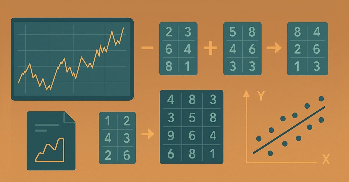
Matrix factorization is a mathematical technique used to decompose a large matrix into a product of smaller, simpler matrices. These techniques come with many benefits. However, before exploring those, let’s first understand the motivation behind them.

In everyday life, certain shared experiences transcend cultures. For example, I believe most readers are familiar with the idea that by talking to a child and listening to how they describe their parent, we can get an idea of what that parent might be like. These descriptions may even help us guess how the parent would act in situations the child hasn’t directly described. Similarly, matrix factorization breaks down a large matrix into smaller ones—its “children.” These child matrices each describe different aspects of the original matrix, helping us understand its underlying structure. Just as a child’s perspective can reveal the essence of their parent, these smaller matrices can reveal in-depth insights about the market we’re analyzing.

The results of matrix factorization often provide numerically stable solutions to the linear models we introduced earlier. In this article, we’ll also introduce a numerical library called OpenBLAS—short for Basic Linear Algebra Subprograms. OpenBLAS is an open-source fork of the BLAS library, redesigned to run efficiently on today’s computational architectures. BLAS was originally written in Fortran and hand-written assembly code.

It is a foundational concept in linear algebra that any dataset can be broken down into smaller components, and these components can be used to build predictive models of the original data. The representations given by these smaller datasets may also reveal characteristics of the original data that would otherwise remain hidden.

This article will gently introduce you to powerful linear algebra commands used to build predictive models from raw data. And that’s just the beginning. These matrix factorization techniques offer much more than raw predictive power—they also help us compress data, uncover hidden trends, and assess market stability or chaos. It’s truly remarkable how much insight we can gain from any dataset—simply by factorizing it. Let’s get started.

Getting Started in MQL5

The first step in getting started with MQL5 is to define the system constants we’ll use throughout this demonstration. These constants support the script I’ve built to get us up and running with matrix factorization.

//+------------------------------------------------------------------+
//|                                                        Solve.mq5 |
//|                                               Gamuchirai Ndawana |
//|                    https://www.mql5.com/en/users/gamuchiraindawa |
//+------------------------------------------------------------------+
#property copyright "Gamuchirai Ndawana"
#property link      "https://www.mql5.com/en/users/gamuchiraindawa"
#property version   "1.00"
#property script_show_inputs

//+------------------------------------------------------------------+
//| System definitions                                               |
//+------------------------------------------------------------------+
#define HORIZON 10
#define START   0

Next, we define the user inputs for the script—specifically how many bars of information we wish to fetch.

//+------------------------------------------------------------------+
//| User inputs                                                      |
//+------------------------------------------------------------------+
input int FETCH =  10;//How many bars should we fetch?

Following that, we declare our global variables, which include training and test data, along with a few others to store the coefficients learned by our application from the data we provide.

//+------------------------------------------------------------------+
//| Global variables                                                 |
//+------------------------------------------------------------------+
int ROWS        =   5;
//Dependent variable
matrix y,y_test;
//Indenpendent variable
matrix X = matrix::Ones(ROWS,FETCH);
matrix X_test = matrix::Ones(ROWS,FETCH);
//Coefficients
matrix b;
vector temp;
//Row Norms
vector row_norms = vector::Zeros(4);
vector error_vector = vector::Zeros(4);

To begin, we print the input data matrix X as it currently stands. As shown in Figure 1, this matrix is initially filled with ones. This is deliberate: in a linear model, the first row of inputs represents the intercept term. Actual market data—such as the opening, high, low, and closing prices—will populate the matrix starting from the second row.

A key point worth mentioning is the layout of the data. If you’ve been following our series, such as Reimagining Classic Strategies, where we extract data from MetaTrader 5 and process it in Python, you may be used to the format where columns represent market attributes (open, high, low, close) and rows represent time (e.g., days). However, in this case, the layout is transposed: time runs along the columns, while market features like open, high, low, and close run along the rows.

//+------------------------------------------------------------------+
//| Script program start function                                    |
//+------------------------------------------------------------------+
void OnStart()
  {
//--- Observe the input matrix in its original form
PrintFormat("Input Matrix Gathered From %s",Symbol());
Print(X);

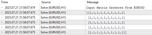
Figure 1: Visualizing our current EURUSD input data from the market

With that clarified, we move on to the part of the script responsible for fetching historical market data. After fetching, we store the norm of each vector and then divide each vector by its norm. This normalization step ensures each vector has a length of 1, a crucial requirement before applying any form of matrix factorization.

Why normalize? Matrix factorization seeks to understand in which direction a matrix is growing and compares growth rates across rows and columns. To make these comparisons fair, we convert each row into a unit vector by dividing it by its norm.

//--- Fetch the data
temp.CopyRates(Symbol(),PERIOD_CURRENT,COPY_RATES_OPEN,START+HORIZON+(FETCH*2),FETCH);
row_norms[0] = temp.Norm(VECTOR_NORM_P);
X.Row(temp/row_norms[0],1);

temp.CopyRates(Symbol(),PERIOD_CURRENT,COPY_RATES_HIGH,START+HORIZON+(FETCH*2),FETCH);
row_norms[1] = temp.Norm(VECTOR_NORM_P);
X.Row(temp/row_norms[1],2);

temp.CopyRates(Symbol(),PERIOD_CURRENT,COPY_RATES_LOW,START+HORIZON+(FETCH*2),FETCH);
row_norms[2] = temp.Norm(VECTOR_NORM_P);
X.Row(temp/row_norms[2],3);

temp.CopyRates(Symbol(),PERIOD_CURRENT,COPY_RATES_CLOSE,START+HORIZON+(FETCH*2),FETCH);
row_norms[3] = temp.Norm(VECTOR_NORM_P);
X.Row(temp/row_norms[3],4);

//--- Fetch the test data
temp.CopyRates(Symbol(),PERIOD_CURRENT,COPY_RATES_OPEN,START+HORIZON+(FETCH),FETCH);
X_test.Row(temp/row_norms[0],1);

temp.CopyRates(Symbol(),PERIOD_CURRENT,COPY_RATES_HIGH,START+HORIZON+(FETCH),FETCH);
X_test.Row(temp/row_norms[1],2);

temp.CopyRates(Symbol(),PERIOD_CURRENT,COPY_RATES_LOW,START+HORIZON+(FETCH),FETCH);
X_test.Row(temp/row_norms[2],3);

temp.CopyRates(Symbol(),PERIOD_CURRENT,COPY_RATES_CLOSE,START+HORIZON+(FETCH),FETCH);
X_test.Row(temp/row_norms[3],4);

When we print the input training data, the first row contains ones—representing the intercept—followed by rows for open, high, low, close, and finally the moving average. The data starts around 0.3 because of normalization.

//--- The train data
Print("Input");
Print(X);

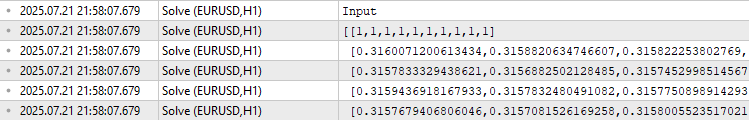
Figure 2: Visualizing our training data after normalizing each row by its vector norm

Next, we define our targets. In this example, the target is the closing price, which we copy into matrix y. Now, X contains our input features, and y contains the values we aim to predict.

//--- Fill the target 
y.CopyRates(Symbol(),PERIOD_CURRENT,COPY_RATES_CLOSE,START+(FETCH*2),FETCH);
y_test.CopyRates(Symbol(),PERIOD_CURRENT,COPY_RATES_CLOSE,START,FETCH);

Print("Target");
Print(y);

Figure 3: The output values we were trying to predict from the past market observations we had on hand

So how do we find coefficients that map X to y? It turns out that infinitely many coefficient sets can do this, so we need a way to choose the most appropriate one. Typically, we select the coefficients that minimize the error between the predicted and actual target values. One well-known method for achieving this is by using the pseudo-inverse.

To compute the coefficients, we multiply the pseudo-inverse of X by y. This matrix multiplication yields the best-fit coefficients in closed form. Thankfully, MQL5 provides a built-in function for this using the PInv() (pseudo-inverse) function.

Do not allow the simplicity of this solution to fool you. I could easily dedicate the remainder of this entire article just to explain the signficance of this one line of code. The solution of coefficients generated by the MQL5 PInv() function is gaurenteed to best minimize the RMSE error between the predictions and the past observations. Moreover, these solutions are gaurenteed to exist. The algorithm is numerically stable and offers us a compact and easily maintainable codebase for building your own predictive models directly from raw data. But this is not the recommended solution you should use.

//--- More Penrose Psuedo Inverse Solution implemented by MQL5 Developers
b = y.MatMul(X.PInv());

Print("Pseudo Inverse Solution: ");
Print(b);

Figure 4: The coefficients produced by matrix multiplying our target and the Psuedo Inverse of our inputs, are the coefficients that will minimize our error

This article’s goal is to introduce you to OpenBLAS and other matrix factorizations. So, why should we learn OpenBLAS if MQL5 already provides a simple way to build predictive models just by using the coefficients computed by the PInv() function? There are several compelling reasons, chief among them being speed. OpenBLAS is astronomically faster than MQL5’s built-in pseudo-inverse. Learning how to use it will drastically increase the speed of your backtests.

Unsupervised Matrix Factorization: Singular Value Decomposition

As mentioned in the introduction, any given data matrix can be broken down into the product of smaller matrices. These smaller matrices can be thought of as "children" of the original matrix, each offering a unique description of their "parent."

The Singular Value Decomposition (SVD) algorithm is one of many ways to factorize a matrix. SVD—short for Singular Value Decomposition—breaks any matrix into the product of three smaller, elementary matrices. Each of these three matrices captures a distinct characteristic of the original matrix. In this section, we’ll get to know each of these three "children" from the SVD factorization. We’ll explore the motivation behind SVD, and what each component can reveal about the original matrix.

Before we dive in, it’s important to clarify the terminology. You may have seen the term unsupervised matrix factorization used alongside matrix factorization, but the two are not interchangeable. Unsupervised matrix factorization is a specific type of factorization technique. It differs from general factorization by focusing only on the most relevant components of the data.

In essence, unsupervised matrix factorization doesn’t return all the children to us—it returns only the most important ones. The algorithm decomposes the matrix and then uses its own internal criteria to decide which factors (or children) are most valuable. This decision is made in an unsupervised way, meaning the algorithm does not rely on labeled outputs or human input to determine relevance. We don’t choose which children to meet—the algorithm decides for us.

As illustrated in Figure 5, SVD is one such matrix factorization method, that decomposes any matrix A into the output of 3 of its "children".

OpenBLAS allows the SVD method to return all "children", or just the most important "children" matrices, it is all dependent on the parameters passed to the SVD call.

In this discussion, we will instruct the OpenBLAS library to only return the most important "children" matrices to us, hence the title of our discussion "Unsupervised Matrix Factorization". As we have already stated, SVD will decompose our original matrix, into the product of 3 simpler, elementary matrices. We’ll now discuss each of these 3 components in turn.

Figure 5: Visualizing the SVD factorization

U is describing hidden market forces that appear to be "driving" our market's observed behaivour. These hidden forces, are more appropriately reffered to as factors. So the first column of U informs us of a market driving force, that depreciates all 4 OHLC prices whenever this force dominates the market. The second market force is dominated by positive coefficients, meaning it has an overall bullish effect on the market. Given that we are working with historical market data, these market forces we are analyzing, may actually represent underlying investor sentiment.

//--- Native MQL5 SVD Solution are also possible without relying on OpenBLAS
Print("Computing Singular Value Decomposition using MQL5");
matrix U,VT;
vector S;
X.SVD(U,VT,S);

Print("U");
Print(U);

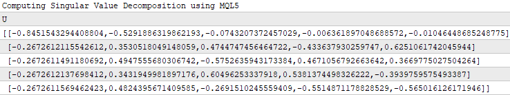
Figure 6: Understanding the "U" component of SVD

V is describing to us how strong each of the forces in U is pronounced along all the time observations in the original dataset. So for example, if we consider the first row of V, we can see that the largest entry is 0.4262. This value is in the 3rd column of the first row of V, meaning that the 3rd column of U describes the force that dominated the market on the first historical day of trading. The 3rd column of U describes a mixed force that negatively affects some components of price, and positively affects others. Such forces may be intermittent, or weak.

Print("VT");
Print(VT);

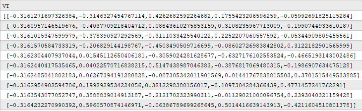
Figure 7: Understnading how pronounced each of the market driving forces are at each time

The Sigma factor informs us on the importance levels of each of the market forces, described in U. The force that dominates our historical observations is assigned the largest the largest value in Sigma, forces that are less pronounced in the data, are assigned smaller values in Sigma. Therefore, we can clearly see that 3.741 is the largest value in Sigma, and this value is in the first column of Sigma, this means that the first column of U, describes the most dominant market force observed in the data.

Print("S");
Print(S);

Figure 8: Understanding the Sigma factor from the SVD factorization

This discussion is not intended to be exhaustive, there is still a lot more that can be said about the 3 factors,U,S and V. In Figures 6,7 and 8, we analyzed what was returned when we called the SVD method natively built in to MQL5. These results closely match what is returned when we call SingularValueDecompositionDC() from the OpenBLAS library.

In Figure 9 below, we have included a screenshot of the U factor when calculated with OpenBLAS, the reader can compare Figure 9 and Figure 6 to learn that both the native MQL5 function and the OpenBLAS function calculate approximately the same U factor. Due to differences in the functions being implementated under the hood, the 2 figures do not match down to the last decimal point, but this is understandable.

//--- OpenBLAS SVD Solution, considerably powerful substitute to the closed solution provided by the MQL5 developers 
matrix OB_U,OB_VT,OB_SIGMA;
vector OB_S;

//--- Perform truncated SVD, we will explore what 'truncated' means later.
PrintFormat("Computing Singular Value Decomposition of %s Data using OpenBLAS",Symbol());
X.SingularValueDecompositionDC(SVDZ_S,OB_S,OB_U,OB_VT);

//--- U is a unitary matrix that is of dimension (m,r)
Print("Open BLAS U");
Print(OB_U);

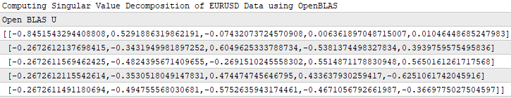
Figure 9: The U factor as calculated by OpenBLAS

In Figure 4 above, we demonstrated that the MQL5 PInv() function, will always give us the coeffecients that map the inputs to the target with the lowest error possible. I will stress this point again, do not allow the simplicity of the solution provided in Figure 4, to fool you. It is a mathematically powerful solution that is gaurenteed to exist for any arbitrary matrix A, and it will also minimize the L2 norm of the matrix Ax-b.

What we did not mention above Figure 4 was that, the PInv() function could really just be calling the SVD() function, on your behalf. Mathemtically speaking, the Psuedo inverse is normally calculated using the Singular Value Decomposition of the original data. Let us see this for ourselves.

In the code snippet below, I have taken the 3 children matrices that we stored when we called SVD() on our market data. We will not expliclity go over all the rules of linear algebra that the reader needs to understand, neither will we attempt to derive this solution, but I only wish to demonstrate that I can obtain linear coefficients that map my input data and my target easily by using the children matrices that SVD returned to me.

Print("Comparing OLS Solutions");
Print("Native MQL5 Solution");
//--- We will always benchmark the native solution as the truth, the MQL5 developers implemented an extremely performant benchmark for us
Print(b);

//--- The OpenBLAS solution came closest to the native solution implemented for us
Print("OpenBLAS Solution");
matrix ob_solution = y.MatMul(OB_VT.Transpose().MatMul(OB_SIGMA.Inv()).MatMul(OB_U.Transpose()));
Print(ob_solution);

//--- Our manual solution was not even close! We will therefore rely on the OpenBLAS solution.
Print("Manual SVD Solution");
matrix svd_solution = y.MatMul(VT).MatMul(SIGMA.Inv()).MatMul(U.Transpose());
Print(svd_solution);

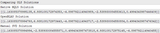
Figure 10: The coefficients that best map my input data and my output data can be obtained by SVD

If the reader is observant, then you lilkely noticed that none of the set of coefficents in Figure 10 precisely match each other. This is to be expected, recall that we used 3 different functions to obtain each set of coefficents. This is akin to having 3 independent students who each perform their homework using their own internal methods. However, what matters more to us, is the error that these coefficents will produce when we use them to make predicitons on data we did not use to train the model.

As we can see in Figure 11, the OpenBLAS SVD solution, produced the lowest error when predicting the test data. However, I want to make sure the reader does not confuse Figure 11 to be the motivation for introducing OpenBLAS.

Notice that all 3 error levels are moderately close to each other. Therefore, if we repeat this test multiple times, on different markets, fetching different amounts of data on each testing round, then OpenBLAS may not always produce the lowest erro. I want the reader to understand that the OpenBLAS library is attractive to us because it is carefully optimized and actively maintained to be fast and reliable. It is not gaurenteed to always produce the lowest error, no single library can make such broad claim.

//--- Measuring the amount of error
//--- Information lost by MQL5 PsuedoInverse solution
//--- The Frobenius norm squares all 
PrintFormat("Information Loss in Forcasting %s Market : ",Symbol());
Print("PInv: ");
matrix pinv_error = ((b.MatMul(X_test)) - y_test);
Print(pinv_error.Norm(MATRIX_NORM_FROBENIUS));

//--- Let the MQL5 implementation be our benchmark
double benchmark = pinv_error.Norm(MATRIX_NORM_FROBENIUS);

//--- Information lost by Manual SVD solution
Print("Manual SVD: ");
matrix svd_error = ((svd_solution.MatMul(X_test)) - y_test);
Print(svd_error.Norm(MATRIX_NORM_FROBENIUS));

//--- Information lost by OpenBLAS SVD solution
Print("OpenBLAS SVD: ");
matrix ob_error = ((ob_solution.MatMul(X_test)) - y_test);
Print(ob_error.Norm(MATRIX_NORM_FROBENIUS));

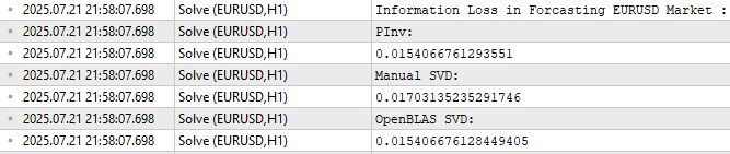
Figure 11: The amount of error produced by each set of coefficients when predicting outside the training period

Appplications of Unsupervised Matrix Factorization Beyond Predictive Modelling

I hope that by this point, my simple presentation style has given you some ideas on what matrix factorization is, and why it may be useful when analyzing financial market data. As I stated earlier, the predictive models we can build using the appropriate matrix factorizations represent only a fraction of the useful tasks we can accomplish using matrix factorization. In this section, I'd like to demonstrate other, useful applications of matrix factorization and how we can incorporate these insights, into our trading applications and strategies.

Matrix Factorization For Unsupervised Market Filtering

I am assuming that the reader has had some personall experience trading, and that from their independent practices they have some understanding for the question I am about to ask. Between, the currency market and the cryptocurrency market, which asset class do you think is more volatile?

I hope the answer was obvious to all of us. Cryptocurrencies are far more volatile than traditional currency markets. For readers who may not be sure what the truth is, we applied the Average True Range (ATR) indicator on the 1 Minute chart of Bitcoin priced in Ethereum on one chart (Figure 12), and the second chart denotes the Euro priced in US dollars below (Figure 13). The ATR indicator measures the volatility in the market, larger ATR readings imply more volatile market conditions. The ATR reading in on the BTCETH chart is approximately 6000% greater than the ATR reading on the EURUSD chart. Therefore, this helps all readers understand why Cryptocurrencies markets are generally considered far more volatile than traditional currency markets.

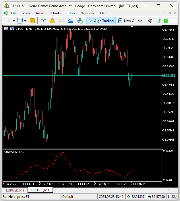
Figure 12: The volaitlity reading of BTCETH is considerably more volatile than EURUSD

Recall that EURUSD is the most liquid currency pair in the world, the EURUSD is the most actively traded currency pair known to man, but its volatility levels pail in comparison to the volatility we observe in the cryptocurrency markets.

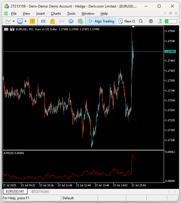
Figure 13:The volatility of traditional asset classes is no match against the volatility produced by cryptocurrency markets

The matrix factorizations we performed earlier could've easily told us the same information. Recall that that in Figure 8, we explained that the factor Sigma, denotes the importance levels of each of the market driving forces appearing in the data. Stable markets, will only have one large entry in the S factor, and all other entries will be close to 0. The more entries in S that are far from 0, the more chaotic and volatile a market appears to be according to the data.

We can apply our script twice, once on the EURUSD market and the second time on the BTCETH market. However, in Figure 14 and 15, both markets appear to be stable. It appears that both markets only have 1 large non-zero entry in S. This would imply that BTCETH is just as stable and well behaved as EURUSD. However, this is not the complete truth of the matter. For us to gain a reliable picture, we must learn another use of matrix factorization.

//+------------------------------------------------------------------+
//| What are we demonstrating here?                                  |
//| 1) We have shown you that any matrix of market data you have,    |
//|    can be analyzed intelligently, to build a linear regression   |
//|    model, using just the raw data.                               |
//| 2) We have demonstrated that the solution to such Linear         |
//|    regression problems, can be obtained through effecient and    |
//|    dedicated functions available in MQL5 or through matrix       |
//|    factorization.                                                |   
//|__________________________________________________________________|
//| I now ask the reader the following question:                     |
//|  "If dedicated functions exist, why bother learning matrix       |
//|   factorization?"                                                |
//+------------------------------------------------------------------+

//--- Matrix factorization gives us a description of the data and it properties
//--- Questions such as: "How stable/chaotic is the market we are in?" can be answered by the factorization we have just performed
//--- Or even questions such as: "How best can I expose the hidden trends in all of this market data?" can still be answered by the factorization we have just performed
//--- I'm only trying to give you a few examples of why you should bother learning these factorizations, even though dedicated functions exist.

//--- Any given matrix A can be represented as the sum of smaller matrices A = USV, this is theorem behind the Singular Value Decomposition.
//--- Each factor is special because each describes different charectersitics of its parent.

//--- Let's get to know Sigma, represented as the S in A = USV.
//--- Sigma technically tells us how many different modes our market appears to exist in, and how important each mode is. 
//--- However, reintepreted in terms of market data, these modes may correspond to investor sentiment.
PrintFormat("Taking a closer look at The Eigenvalues of %s Market Data: ",Symbol());
Print(OB_S/OB_S.Sum());
Print("If sigma has a only few values that are far from 0, then investor's sentiment in this market appears well established and hardly changes");
//--- If Sigma has a lot values that are all far away from 0, then the market is chaotic and it appears investor's sentiment and expectations constantly change
//--- If Sigma has a few, or even just one value that is far away from 0, then investor sentiment in that market appears stable, and hardly changes.
//--- Traders explicitly looking for fast-action scalping oppurtunities may use Sigma as a filter of how much energy the market has. 
//--- Quiet market will have a few dominant values in Sigma, not ideal for scalpers, better suited for long-term trend traders.

Figure 14: Visualizing the amount of energy in the EURUSD market.

Figure 15: Visualizing the amount of energy in the BTCETH market

Matrix Factorization For Data Compression And Signal Extraction

Matrix factorization can also be used to compress data and extract the dominant signal in the data. Since the children matrices are samller than their parent, these algorithms can efficiently compact data. These properties of matrix factorization are well known by any of our fellow community members who may have backgrounds in fields such as networking, signal processing, electrical engineering or other related domains. We can compress our original data by multiplying the S "child" and V "child" matrices. Note that we call the Diag() method on S to convert it into a diagonal matrix, before performing the multiplication. The product of this multiplication is a new and compact representaion of the parent matrix.

The reader may already be familiar with this algorithm, it is commonly known as Principal Component Analysis (PCA). We will not take a deep dive into PCA, rather, I am only trying to demonstrate how much useful information we gain from using matrix factorization. There are many ways to compute the principal components of your market data; matrix factorization using OpenBLAS is likely among the fastest methods available to you natively in MQL5.

//--- Fetch the data and prepare to perform PCA
temp.CopyRates(Symbol(),PERIOD_CURRENT,COPY_RATES_OPEN,START+HORIZON+(FETCH*2),FETCH);
row_norms[0] = temp.Mean();
X.Row(temp-row_norms[0],1);

temp.CopyRates(Symbol(),PERIOD_CURRENT,COPY_RATES_HIGH,START+HORIZON+(FETCH*2),FETCH);
row_norms[1] = temp.Mean();
X.Row(temp-row_norms[1],2);

temp.CopyRates(Symbol(),PERIOD_CURRENT,COPY_RATES_LOW,START+HORIZON+(FETCH*2),FETCH);
row_norms[2] = temp.Mean();
X.Row(temp-row_norms[2],3);

temp.CopyRates(Symbol(),PERIOD_CURRENT,COPY_RATES_CLOSE,START+HORIZON+(FETCH*2),FETCH);
row_norms[3] = temp.Mean();
X.Row(temp-row_norms[3],4);

//--- Fetch the test data
temp.CopyRates(Symbol(),PERIOD_CURRENT,COPY_RATES_OPEN,START+HORIZON+(FETCH),FETCH);
X_test.Row(temp-row_norms[0],1);

temp.CopyRates(Symbol(),PERIOD_CURRENT,COPY_RATES_HIGH,START+HORIZON+(FETCH),FETCH);
X_test.Row(temp-row_norms[1],2);

temp.CopyRates(Symbol(),PERIOD_CURRENT,COPY_RATES_LOW,START+HORIZON+(FETCH),FETCH);
X_test.Row(temp-row_norms[2],3);

temp.CopyRates(Symbol(),PERIOD_CURRENT,COPY_RATES_CLOSE,START+HORIZON+(FETCH),FETCH);
X_test.Row(temp-row_norms[3],4);

//--- Perform truncated SVD, we will explore what 'truncated' means later.
Print("Computing Singular Value Decomposition using OpenBLAS");
X.SingularValueDecompositionDC(SVDZ_S,OB_S,OB_U,OB_VT);

OB_SIGMA.Diag(OB_S);

//--- Calculating Principal Components
Print("Principal Components");
matrix pc = OB_SIGMA.MatMul(OB_VT);
Print(pc);

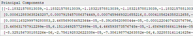
Figure 16: By multiplying the S and V factors, we obtain a compact representation of our original dataset

There is still a lot more that we can discuss about the product produced by multiplying the S and V "children". The product of this multiplication, produces a new representation of our dataset that has considerably less correlation. To prove this, we will compare the norm of the correlation matrix from our original dataset, against the correlation matrix from the product of multiplying S and V. Recal that the norm in Linear Algebra, is analogous to asking "How big" something is. As we can see in Figure 17, the norm of the correlation matrix fell considerably after factorizing the original market data.

This is meant to illustrate to the reader that matrix factorization using SVD can be used to remove redundant correlated features in the original dataset, and hopefully by doing so, we aim to better expose the dominant trends and patterns in the data.

//--- PCA reduces the amount of correlation in our dataset 
Print("How correlated is our new representation of the data?");
//--- First we will measure the size of our original correlation matrix
Print(X.Norm(MATRIX_NORM_FROBENIUS));
//--- Then, we will measure the size of our new correlation matrix produced by factorizing the data
Print(pc.CorrCoef().Norm(MATRIX_NORM_FROBENIUS));

Figure 17: Matrix factorization can help us significantly reduce the amount of correlation in our dataset

Armed with this information, we can build a model of the market that uses only 3 rows of data, instead of the original 5 rows of data we started with. Hopefully these 3 less correlated rows will better explain the relationship between the market and the target, better than the original data. This is called feature extraction, because we are learning new features from the original data. But as with most practices related to optimization, we aren't gaurenteed that this will improve our performance in the future, as depicted in Figure 18.

//--- Main principal components
matrix mpc;

mpc.Row(pc.Row(0),0);
mpc.Row(pc.Row(1),1);
mpc.Row(pc.Row(2),2);

//--- The factor VT describes the correlational structure across the columns of our data
Print("Performing PCA");
matrix pca_coefs = y.MatMul(mpc.PInv());

//--- Performing PCA on the test data
X_test.SingularValueDecompositionDC(SVDZ_S,OB_S,OB_U,OB_VT);
Print("Principal Components of Test Data");
pc = OB_SIGMA.MatMul(OB_VT);

Print(pc);

PrintFormat("Most Important Principal Components in %s Market Test Data",Symbol());
Print(OB_S / OB_S.Sum());

//--- Main principal components
mpc.Row(pc.Row(0),0);
mpc.Row(pc.Row(1),1);
mpc.Row(pc.Row(2),2);

matrix pca_error = pca_coefs.MatMul(mpc) - y_test;

Print("PCA Error: ");
Print(pca_error.Norm(MATRIX_NORM_FROBENIUS));

Print("OpenBLAS Error: ");
Print(ob_error.Norm(MATRIX_NORM_FROBENIUS));

Print("Manual Error: ");
Print(svd_error.Norm(MATRIX_NORM_FROBENIUS));

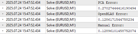
Figure 18: Feature extraction is a powerful numerical method, but it does not gaurentee improved performance

In Figure 14 and 15, we tried to illustrate that matrix factorization can be used to dinguish stable markets from volatile markets. In our first attempt, both markets appeared to only have 1 large value in the S factor. However, after carefully inspecting the data, I learned that this was only true in the train set. If we factorize the test set of our market data, and then analyze the S factor obtained, we can start to see that indeed BTCETH has more "energy" than EURUSD, because BTCETH has 2 entries in S that are far from 0, while EURUSD only has 1.

//--- Performing PCA on the test data
X_test.SingularValueDecompositionDC(SVDZ_S,OB_S,OB_U,OB_VT);
Print("Principal Components of Test Data");
pc = OB_SIGMA.MatMul(OB_VT);


PrintFormat("Most Important Principal Components in %s Market Test Data",Symbol());
Print(OB_S / OB_S.Sum());

Figure 19: Analyzing the amount of energy contained in the EURUSD market

Figure 19: Analyzing the amount of energy contained in the BTCEHTH market. Recall that the more individual entries far from 0 that you observe, the more chaotic the market is

All in our this is the MQL5 script that I prepared for our dicussion on unsupervised matrix factorization.

//+------------------------------------------------------------------+
//|                                                        Solve.mq5 |
//|                                               Gamuchirai Ndawana |
//|                    https://www.mql5.com/en/users/gamuchiraindawa |
//+------------------------------------------------------------------+
#property copyright "Gamuchirai Ndawana"
#property link      "https://www.mql5.com/en/users/gamuchiraindawa"
#property version   "1.00"
#property script_show_inputs

//+------------------------------------------------------------------+
//| System definitions                                               |
//+------------------------------------------------------------------+
#define HORIZON 10
#define START   0

//+------------------------------------------------------------------+
//| User inputs                                                      |
//+------------------------------------------------------------------+
input int FETCH =  10;//How many bars should we fetch?

//+------------------------------------------------------------------+
//| Global variables                                                 |
//+------------------------------------------------------------------+
int ROWS        =   5;
//Dependent variable
matrix y,y_test;
//Indenpendent variable
matrix X = matrix::Ones(ROWS,FETCH);
matrix X_test = matrix::Ones(ROWS,FETCH);
//Coefficients
matrix b;
vector temp;
//Row Norms
vector row_norms = vector::Zeros(4);
vector error_vector = vector::Zeros(4);

//+------------------------------------------------------------------+
//| Script program start function                                    |
//+------------------------------------------------------------------+
void OnStart()
  {
//--- Observe the input matrix in its original form
PrintFormat("Input Matrix Gathered From %s",Symbol());
Print(X);
  
//--- Fetch the data
temp.CopyRates(Symbol(),PERIOD_CURRENT,COPY_RATES_OPEN,START+HORIZON+(FETCH*2),FETCH);
row_norms[0] = temp.Norm(VECTOR_NORM_P);
X.Row(temp/row_norms[0],1);

temp.CopyRates(Symbol(),PERIOD_CURRENT,COPY_RATES_HIGH,START+HORIZON+(FETCH*2),FETCH);
row_norms[1] = temp.Norm(VECTOR_NORM_P);
X.Row(temp/row_norms[1],2);

temp.CopyRates(Symbol(),PERIOD_CURRENT,COPY_RATES_LOW,START+HORIZON+(FETCH*2),FETCH);
row_norms[2] = temp.Norm(VECTOR_NORM_P);
X.Row(temp/row_norms[2],3);

temp.CopyRates(Symbol(),PERIOD_CURRENT,COPY_RATES_CLOSE,START+HORIZON+(FETCH*2),FETCH);
row_norms[3] = temp.Norm(VECTOR_NORM_P);
X.Row(temp/row_norms[3],4);

//--- Fetch the test data
temp.CopyRates(Symbol(),PERIOD_CURRENT,COPY_RATES_OPEN,START+HORIZON+(FETCH),FETCH);
X_test.Row(temp/row_norms[0],1);

temp.CopyRates(Symbol(),PERIOD_CURRENT,COPY_RATES_HIGH,START+HORIZON+(FETCH),FETCH);
X_test.Row(temp/row_norms[1],2);

temp.CopyRates(Symbol(),PERIOD_CURRENT,COPY_RATES_LOW,START+HORIZON+(FETCH),FETCH);
X_test.Row(temp/row_norms[2],3);

temp.CopyRates(Symbol(),PERIOD_CURRENT,COPY_RATES_CLOSE,START+HORIZON+(FETCH),FETCH);
X_test.Row(temp/row_norms[3],4);

//--- The train data
Print("Input");
Print(X);

//--- Fill the target
y.CopyRates(Symbol(),PERIOD_CURRENT,COPY_RATES_CLOSE,START+(FETCH*2),FETCH);
y_test.CopyRates(Symbol(),PERIOD_CURRENT,COPY_RATES_CLOSE,START,FETCH);

Print("Target");
Print(y);

//--- More Penrose Psuedo Inverse Solution implemented by MQL5 Developers, enterprise level effeciency!
b = y.MatMul(X.PInv());

Print("Pseudo Inverse Solution: ");
Print(b);

//--- Native MQL5 SVD Solution are also possible without relying on OpenBLAS
Print("Computing Singular Value Decomposition using MQL5");
matrix U,VT;
vector S;
X.SVD(U,VT,S);

Print("U");
Print(U);

Print("VT");
Print(VT);

Print("S");
Print(S);
matrix SIGMA;
SIGMA.Diag(S);

//--- OpenBLAS SVD Solution, considerably powerful substitute to the closed solution provided by the MQL5 developers 
matrix OB_U,OB_VT,OB_SIGMA;
vector OB_S;

//--- Perform truncated SVD, we will explore what 'truncated' means later.
PrintFormat("Computing Singular Value Decomposition of %s Data using OpenBLAS",Symbol());
X.SingularValueDecompositionDC(SVDZ_S,OB_S,OB_U,OB_VT);

//--- U is a unitary matrix that is of dimension (m,r)
Print("Open BLAS U");
Print(OB_U);

//--- VT is a mathematically a symmetrical matrix that is (r,r), for effeciency in software it is represented as a vector that is (1,r)
Print("Open BLAS VT");
Print(OB_VT);

//--- We need it in its intended form as an (r,r) matrix, we will explore what this means later. 
Print("Open BLAS S");
Print(OB_S);
OB_SIGMA.Diag(OB_S);

Print("Comparing OLS Solutions");
Print("Native MQL5 Solution");
//--- We will always benchmark the native solution as the truth, the MQL5 developers implemented an extremely performant benchmark for us
Print(b);

//--- The OpenBLAS solution came closest to the native solution implemented for us
Print("OpenBLAS Solution");
matrix ob_solution = y.MatMul(OB_VT.Transpose().MatMul(OB_SIGMA.Inv()).MatMul(OB_U.Transpose()));
Print(ob_solution);

//--- Our manual solution was not even close! We will therefore rely on the OpenBLAS solution.
Print("Manual SVD Solution");
matrix svd_solution = y.MatMul(VT).MatMul(SIGMA.Inv()).MatMul(U.Transpose());
Print(svd_solution);

//--- Measuring the amount of error
//--- Information lost by MQL5 PsuedoInverse solution
//--- The Frobenius norm squares all 
PrintFormat("Information Loss in Forcasting %s Market : ",Symbol());
Print("PInv: ");
matrix pinv_error = ((b.MatMul(X_test)) - y_test);
Print(pinv_error.Norm(MATRIX_NORM_FROBENIUS));

//--- Let the MQL5 implementation be our benchmark
double benchmark = pinv_error.Norm(MATRIX_NORM_FROBENIUS);

//--- Information lost by Manual SVD solution
Print("Manual SVD: ");
matrix svd_error = ((svd_solution.MatMul(X_test)) - y_test);
Print(svd_error.Norm(MATRIX_NORM_FROBENIUS));

//--- Information lost by OpenBLAS SVD solution
Print("OpenBLAS SVD: ");
matrix ob_error = ((ob_solution.MatMul(X_test)) - y_test);
Print(ob_error.Norm(MATRIX_NORM_FROBENIUS));

//+------------------------------------------------------------------+
//| What are we demonstrating here?                                  |
//| 1) We have shown you that any matrix of market data you have,    |
//|    can be analyzed intelligently, to build a linear regression   |
//|    model, using just the raw data.                               |
//| 2) We have demonstrated that the solution to such Linear         |
//|    regression problems, can be obtained through effecient and    |
//|    dedicated functions available in MQL5 or through matrix       |
//|    factorization.                                                |   
//|__________________________________________________________________|
//| I now ask the reader the following question:                     |
//|  "If dedicated functions exist, why bother learning matrix       |
//|   factorization?"                                                |
//+------------------------------------------------------------------+

//--- Matrix factorization gives us a description of the data and it properties
//--- Questions such as: "How stable/chaotic is the market we are in?" can be answered by the factorization we have just performed
//--- Or even questions such as: "How best can I expose the hidden trends in all of this market data?" can still be answered by the factorization we have just performed
//--- I'm only trying to give you a few examples of why you should bother learning these factorizations, even though dedicated functions exist.

//--- Any given matrix A can be represented as the sum of smaller matrices A = USV, this is theorem behind the Singular Value Decomposition.
//--- Each factor is special because each describes different charectersitics of its parent.

//--- Let's get to know Sigma, represented as the S in A = USV.
//--- Sigma technically tells us how many different modes our market appears to exist in, and how important each mode is. 
//--- However, reintepreted in terms of market data, these modes may correspond to investor sentiment.
PrintFormat("Taking a closer look at The Eigenvalues of %s Market Data: ",Symbol());
Print(OB_S/OB_S.Sum());
Print("If sigma has a only few values that are far from 0, then investor's sentiment in this market appears well established and hardly changes");
//--- If Sigma has a lot values that are all far away from 0, then the market is chaotic and it appears investor's sentiment and expectations constantly change
//--- If Sigma has a few, or even just one value that is far away from 0, then investor sentiment in that market appears stable, and hardly changes.
//--- Traders explicitly looking for fast-action scalping oppurtunities may use Sigma as a filter of how much energy the market has. 
//--- Quiet market will have a few dominant values in Sigma, not ideal for scalpers, better suited for long-term trend traders.

//--- Fetch the data and prepare to perform PCA
temp.CopyRates(Symbol(),PERIOD_CURRENT,COPY_RATES_OPEN,START+HORIZON+(FETCH*2),FETCH);
row_norms[0] = temp.Mean();
X.Row(temp-row_norms[0],1);

temp.CopyRates(Symbol(),PERIOD_CURRENT,COPY_RATES_HIGH,START+HORIZON+(FETCH*2),FETCH);
row_norms[1] = temp.Mean();
X.Row(temp-row_norms[1],2);

temp.CopyRates(Symbol(),PERIOD_CURRENT,COPY_RATES_LOW,START+HORIZON+(FETCH*2),FETCH);
row_norms[2] = temp.Mean();
X.Row(temp-row_norms[2],3);

temp.CopyRates(Symbol(),PERIOD_CURRENT,COPY_RATES_CLOSE,START+HORIZON+(FETCH*2),FETCH);
row_norms[3] = temp.Mean();
X.Row(temp-row_norms[3],4);

//--- Fetch the test data
temp.CopyRates(Symbol(),PERIOD_CURRENT,COPY_RATES_OPEN,START+HORIZON+(FETCH),FETCH);
X_test.Row(temp-row_norms[0],1);

temp.CopyRates(Symbol(),PERIOD_CURRENT,COPY_RATES_HIGH,START+HORIZON+(FETCH),FETCH);
X_test.Row(temp-row_norms[1],2);

temp.CopyRates(Symbol(),PERIOD_CURRENT,COPY_RATES_LOW,START+HORIZON+(FETCH),FETCH);
X_test.Row(temp-row_norms[2],3);

temp.CopyRates(Symbol(),PERIOD_CURRENT,COPY_RATES_CLOSE,START+HORIZON+(FETCH),FETCH);
X_test.Row(temp-row_norms[3],4);

//--- Perform truncated SVD, we will explore what 'truncated' means later.
Print("Computing Singular Value Decomposition using OpenBLAS");
X.SingularValueDecompositionDC(SVDZ_S,OB_S,OB_U,OB_VT);

//--- Calculating Principal Components
Print("Principal Components");
matrix pc = OB_SIGMA.MatMul(OB_VT);
Print(pc);

PrintFormat("Most Important Principal Components of %s Market Data",Symbol());
Print(OB_S / OB_S.Sum());

//--- Main principal components
matrix mpc;

mpc.Row(pc.Row(0),0);
mpc.Row(pc.Row(1),1);
mpc.Row(pc.Row(2),2);

//--- The factor VT describes the correlational structure across the columns of our data
Print("Performing PCA");
matrix pca_coefs = y.MatMul(mpc.PInv());

//--- Performing PCA on the test data
X_test.SingularValueDecompositionDC(SVDZ_S,OB_S,OB_U,OB_VT);
Print("Principal Components of Test Data");
pc = OB_SIGMA.MatMul(OB_VT);

Print(pc);

PrintFormat("Most Important Principal Components in %s Market Test Data",Symbol());
Print(OB_S / OB_S.Sum());

//--- Main principal components
mpc.Row(pc.Row(0),0);
mpc.Row(pc.Row(1),1);
mpc.Row(pc.Row(2),2);

matrix pca_error = pca_coefs.MatMul(mpc) - y_test;

Print("PCA Error: ");
Print(pca_error.Norm(MATRIX_NORM_FROBENIUS));

Print("OpenBLAS Error: ");
Print(ob_error.Norm(MATRIX_NORM_FROBENIUS));

Print("Manual Error: ");
Print(svd_error.Norm(MATRIX_NORM_FROBENIUS));

}
//+------------------------------------------------------------------+

Building Our Application

We will start combining what we have discussed so far into a single trading strategy. Our strategy aims to learn a fair market price by forecasting the moving average indicator's future value. This expected value is going to help us place our trades in the sense that, when price levels are above our expectations, we will sell because we believe the market is overvalued, the opposite is true for our long positions.

Let us apply a 10 period moving average on the EURUSD Daily chart, and shift it forward to imagine its shifted value as our prediction.

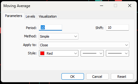
Figure 20: For illustrative purposes, we simply shifted the moving average indicator forward 10 steps

Our trading strategy essentially assumes that current price levels will eventually align with the expected value. In the setup depicted in Figure 21, the expected price is low while the current price is high. Suppose Figure 21 was generated by our market prediction—this would be our signal.

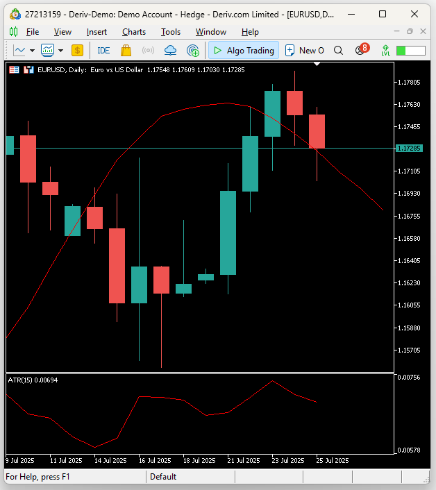
Figure 21: Visualizing our trading strategy, the shifted moving average implies we will trade based on where our model anticipates the moving average to be

Establishing A Baseline

Before building our application, we must establish a baseline to evaluate the performance of our AI model. This baseline will demonstrate the expected outcome without using AI. Since we will explore the full implementation of our application in the following sections, I will now briefly highlight the key elements of the baseline.

//+------------------------------------------------------------------+
//| Obtain a prediction from our model                               |
//+------------------------------------------------------------------+
void setup(void)
  {
   y.CopyIndicatorBuffer(ma_close_handler,0,0,bars);
   
   Print("Training Target");
   Print(y);

//--- Get a prediction
   prediction = y.Mean();
   Print("Prediction");
   Print(prediction);
  }
//+------------------------------------------------------------------+

The baseline makes its predictions by replicating moving average indicator values—calculating their mean and trading based on that. If the mean value of the moving average indicator exceeds the current price, we buy; otherwise, we sell.

if(prediction > c)
  {
   Trade.Buy(TradeInformation.MinVolume(),Symbol(),TradeInformation.GetAsk(),proposed_buy_sl,0);
   state = 1;
  }
if(prediction < c)
  {
   Trade.Sell(TradeInformation.MinVolume(),Symbol(),TradeInformation.GetBid(),proposed_sell_sl,0);
   state = -1;
  }

We will now apply our application to the USD/UL pair, as shown in Figure 22, using two years of historical data from January 2023 to March 2025.

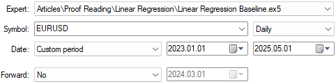
Figure 22: Testing our baseline application on historical market data

Figure 23 displays the application settings we are using. It is important to keep these input settings fixed across tests to ensure fair comparisons.

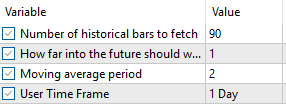
Figure 23: We will keep our benchmark parameters fixed to ensure fair compairsons

Figure 24 presents the equity curve produced by our trading strategy. The results show that our approach is sound, with the account balance trending positively over time.

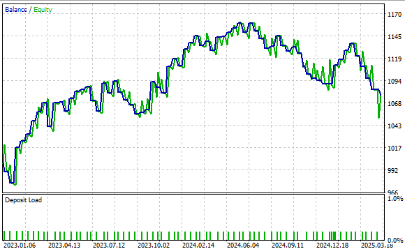
Figure 24: Our benchmark application has set a strong performance level for us to outperform with our new understanding of matrix factorization

Figure 25 provides detailed performance metrics. The strategy achieved a 51% win rate, showing consistent profitability. It produced a positive Sharpe ratio of 0.47—a healthy value. While further refinements may enhance this ratio, the system already provides a strong benchmark. Even with naive predictions of future moving average values, we can construct a profitable strategy. Now, let us explore the benefits of making more informed predictions.

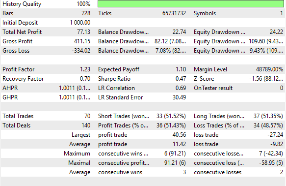
Figure 25: Detailed analysis of our benchmark performance levels

Improving Our Results

We’re now ready to begin building our application and the MQL5. We'll start by defining the key system constants needed so far. These constants will control the technical indicators our system will rely on, as well as define the total number of inputs required by the application.

//+------------------------------------------------------------------+
//|                                            Linear Regression.mq5 |
//|                                               Gamuchirai Ndawana |
//|                    https://www.mql5.com/en/users/gamuchiraindawa |
//+------------------------------------------------------------------+
#property copyright "Gamuchirai Ndawana"
#property link      "https://www.mql5.com/en/users/gamuchiraindawa"
#property version   "1.00"

//+------------------------------------------------------------------+
//| System constants                                                 |
//+------------------------------------------------------------------+
#define TOTAL_INPUTS 6

Next, we’ll define system inputs that users can tune to modify the system’s behavior,.

//+------------------------------------------------------------------+
//| System Inputs                                                    |
//+------------------------------------------------------------------+
input int bars = 10;//Number of historical bars to fetch
input int horizon = 10;//How far into the future should we forecast
input int MA_PERIOD = 24; //Moving average period
input ENUM_TIMEFRAMES TIME_FRAME = PERIOD_H1;//User Time Frame

We will also declare a set of important global variables to track all the parameters used by our linear regression model.

//+------------------------------------------------------------------+
//| Dependencies                                                     |
//+------------------------------------------------------------------+
#include <Trade\Trade.mqh>
#include <VolatilityDoctor\Time\Time.mqh>
#include <VolatilityDoctor\Trade\TradeInfo.mqh>

During the initialization sequence of our Expert Advisor, we will instantiate all global variables with their default values and initialize the relevant technical indicators.

//+------------------------------------------------------------------+
//| Global Variables                                                 |
//+------------------------------------------------------------------+
int        ma_close_handler;
double     ma_close[];
Time       *Timer;
TradeInfo  *TradeInformation;
vector     bias,temp,Z1,Z2;
matrix     X,y,prediction,b;
int        time;
CTrade Trade;
int state;
int atr_handler;
double atr[];

In the deinitialization sequence, we will free up any space previously assigned to global variables, including any technical indicators that are no longer needed.

//+------------------------------------------------------------------+
//| Expert initialization function                                   |
//+------------------------------------------------------------------+
int OnInit()
  {
//---
   Timer            = new Time(Symbol(),TIME_FRAME);
   TradeInformation        = new TradeInfo(Symbol(),TIME_FRAME);
   ma_close_handler = iMA(Symbol(),TIME_FRAME,MA_PERIOD,0,MODE_SMA,PRICE_CLOSE);
   bias = vector::Ones(TOTAL_INPUTS);
   Z1 = vector::Ones(TOTAL_INPUTS);
   Z2 = vector::Ones(TOTAL_INPUTS);
   X = matrix::Ones(TOTAL_INPUTS,bars);
   y = matrix::Ones(1,bars);
   time = 0;
   state = 0;
   atr_handler = iATR(Symbol(),TIME_FRAME,14);
//---
   return(INIT_SUCCEEDED);
  }

When updated price levels are received by our application, we want to appropriately adjust the weights of our model's coefficients and keep them closely tracking current market conditions. This means we will be calculating the SVD factorization a considerable number of times, during our backtest. However, this is the virtue of the fasy implementation provided to us by the OpenBLAS team. The multiple calls we will make, barely slow down the speed of our historical backtests.

//+------------------------------------------------------------------+
//| Expert tick function                                             |
//+------------------------------------------------------------------+
void OnTick()
  {
//---
   if(Timer.NewCandle())
     {
      setup();
      double c =  iClose(Symbol(),TIME_FRAME,0);
      CopyBuffer(atr_handler,0,0,1,atr);
      CopyBuffer(ma_close_handler,0,0,1,ma_close);

      if(PositionsTotal() == 0)
        {
         state = 0;
         if(prediction[0,0] > c)
           {
            Trade.Buy(TradeInformation.MinVolume(),Symbol(),TradeInformation.GetAsk(),(TradeInformation.GetBid() - (2 * atr[0])),0);
            state = 1;
           }
         if(prediction[0,0] < c)
           {
            Trade.Sell(TradeInformation.MinVolume(),Symbol(),TradeInformation.GetBid(),(TradeInformation.GetAsk() + (2 * atr[0])),0);
            state = -1;
           }
        }

      if(PositionsTotal() > 0)
        {
         if(((state == -1) && (prediction[0,0] > c)) || ((state == 1)&&(prediction[0,0] < c)))
            Trade.PositionClose(Symbol());
            if(PositionSelect(Symbol()))
               {
                  double current_sl = PositionGetDouble(POSITION_SL);
                  
                  if((state == 1) && ((ma_close[0] - (2 * atr[0]))>current_sl))
                     {
                        Trade.PositionModify(Symbol(),(ma_close[0] - (2 * atr[0])),0);
                     }
                     
                  else if((state == -1) && ((ma_close[0] + (1 * atr[0]))<current_sl))
                     {
                        Trade.PositionModify(Symbol(),(ma_close[0] + (2 * atr[0])),0);
                     }
               }
        }
     }
  }

Finally, we define the function used to obtain predictions from our linear regression model using the standardized and scaled Z-values tracked in vectors named Z1 (for the mean) and Z2 (for the standard deviation). Each of these scaled row vectors is stored in the X_inputs matrix, and the associated moving average value we aim to predict is stored in Y. We then fit the model using the factorization methods previously described and use the learned coefficients to make predictions.

//+------------------------------------------------------------------+
//| Obtain a prediction from our model                               |
//+------------------------------------------------------------------+
void setup(void)
  {

//--- OpenBLAS SVD Solution, considerably powerful substitute to the closed solution provided by the MQL5 developers 
matrix OB_U,OB_VT,OB_SIGMA;
vector OB_S;

//--- Reshape the matrix
   X = matrix::Ones(TOTAL_INPUTS,bars);

//--- Store the Z-scores
   temp.CopyRates(Symbol(),TIME_FRAME,COPY_RATES_OPEN,horizon,bars);
   Z1[0] = temp.Mean();
   Z2[0] = temp.Std();
   temp = ((temp - Z1[0]) / Z2[0]);
   X.Row(temp,1);

//--- Store the Z-scores
   temp.CopyRates(Symbol(),TIME_FRAME,COPY_RATES_HIGH,horizon,bars);
   Z1[1] = temp.Mean();
   Z2[1] = temp.Std();
   temp = ((temp - Z1[1]) / Z2[1]);
   X.Row(temp,2);

//--- Store the Z-scores
   temp.CopyRates(Symbol(),TIME_FRAME,COPY_RATES_LOW,horizon,bars);
   Z1[2] = temp.Mean();
   Z2[2] = temp.Std();
   temp = ((temp - Z1[2]) / Z2[2]);
   X.Row(temp,3);

//--- Store the Z-scores
   temp.CopyRates(Symbol(),TIME_FRAME,COPY_RATES_CLOSE,horizon,bars);
   Z1[3] = temp.Mean();
   Z2[3] = temp.Std();
   temp = ((temp - Z1[3]) / Z2[3]);
   X.Row(temp,4);

//--- Store the Z-scores
   temp.CopyIndicatorBuffer(ma_close_handler,0,horizon,bars);
   Z1[4] = temp.Mean();
   Z2[4] = temp.Std();
   temp = ((temp - Z1[4]) / Z2[4]);
   X.Row(temp,5);

   temp.CopyIndicatorBuffer(ma_close_handler,0,0,bars);
   y.Row(temp,0);
   
   Print("Training Input Data: ");
   Print(X);

   Print("Training Target");
   Print(y);

//--- Perform truncated SVD, we will explore what 'truncated' means later.
PrintFormat("Computing Singular Value Decomposition of %s Data using OpenBLAS",Symbol());
X.SingularValueDecompositionDC(SVDZ_S,OB_S,OB_U,OB_VT);
OB_SIGMA.Diag(OB_S);

//--- Fit the model
//--- More Penrose Psuedo Inverse Solution implemented by MQL5 Developers, enterprise level effeciency!
   b = y.MatMul(OB_VT.Transpose().MatMul(OB_SIGMA.Inv()).MatMul(OB_U.Transpose()));
   Print("OLS Solutions: ");
   Print(b);

//--- Prepare to get a prediction
//--- Reshape the data
   X = matrix::Ones(TOTAL_INPUTS,1);

//--- Get a prediction
   temp.CopyRates(Symbol(),TIME_FRAME,COPY_RATES_OPEN,0,1);
   temp = ((temp - Z1[0]) / Z2[0]);
   X.Row(temp,1);

   temp.CopyRates(Symbol(),TIME_FRAME,COPY_RATES_HIGH,0,1);
   temp = ((temp - Z1[1]) / Z2[1]);
   X.Row(temp,2);

   temp.CopyRates(Symbol(),TIME_FRAME,COPY_RATES_LOW,0,1);
   temp = ((temp - Z1[2]) / Z2[2]);
   X.Row(temp,3);

   temp.CopyRates(Symbol(),TIME_FRAME,COPY_RATES_CLOSE,0,1);
   temp = ((temp - Z1[3]) / Z2[3]);
   X.Row(temp,4);

   temp.CopyIndicatorBuffer(ma_close_handler,0,0,1);
   temp = ((temp - Z1[4]) / Z2[4]);
   X.Row(temp,5);

   Print("Prediction Inputs: ");
   Print(X);

//--- Get a prediction
   prediction = b.MatMul(X);
   Print("Prediction");
   Print(prediction[0,0]);
  }
//+------------------------------------------------------------------+

We are now ready to begin testing the improved version of our trading algorithm. Recall that this implementation is designed to provide better-informed predictions of the expected price value. We will keep the test dates consistent with our initial test, as shown in Figure 26. Also, as illustrated in Figure 23, the application settings remain unchanged. The reader can therefore continue following along using the same configuration.

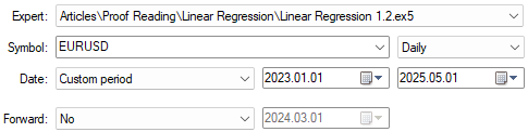
Figure 26: Getting ready to test the improvements realised by our new trading application

Analyzing the new results, we can clearly observe significant improvements. The naive strategy produced a total net profit of $77, whereas our improved strategy achieved a net profit of $101—a notable increase. This represents a 31% growth in total net profit. Additionally, the Sharpe ratio, which was initially 0.47 in the first implementation, has increased to 0.63. This marks a 34% improvement in risk-adjusted returns, indicating meaningful enhancement in the system's performance.

The percentage of profitable trades also increased, rising from 51.4% in the naive system to 51.8% in the improved version. Furthermore, the total number of trades placed grew from 70 to 83, suggesting that the new system is uncovering more trading signals.

While the average size of both winning and losing trades decreased, the system is overall more active and effective. All of this has been achieved using native MQL5 code and by appropriately applying matrix factorizations to the available data.

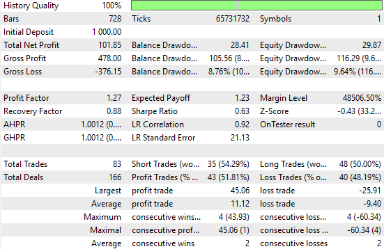
Figure 27: A detailed analysis of the performance levels achieved by our informed predictions of future price levels

We have also included the profit curve produced by our improved version of our trading application. Our new trading system is demonstrating a positive trend in the account balance over historical data, this encourages us to continue seeking further improvents to realise.

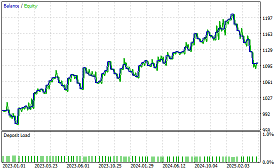
Figure 28: The profit curve produced by our improved trading application

Conclusion

This article has introduced the reader to the many benefits of the MQL5 Matrix API. The API provides powerful mathematical tools that enhance our ability to make informed trading decisions.

Matrix factorizations allow us to uncover patterns hidden in correlated data—patterns that may not be apparent through traditional methods of market analysis. Readers are now equipped with strong alternatives to conventional time series approaches commonly taught in finance. For instance, typical time series analysis begins by differencing the data to measure periodic changes. In contrast, our approach avoided differencing altogether and instead relied on factorizing the data.

This shift in perspective opens the door to a range of applications. We demonstrated how matrix factorization enables fast and numerically stable statistical modeling. It also reduces the dimensionality of the data, simplifying it into more compact forms that better reveal underlying trends.

While much more can be said about the advantages of matrix factorizations, this article provides a solid foundation. Importantly, factorization techniques can reduce the need for explicitly defined trading rules—allowing the system to learn optimal strategies directly from the data.

It is truly remarkable how much we can gain by integrating the MQL5 Matrix API into our daily trading workflows.

Attached files |

Download ZIP

Solve.mq5 (11.9 KB)

Linear_Regression_Baseline.mq5 (5.25 KB)

Linear_Regression_1.2.mq5 (7.85 KB)

Warning: All rights to these materials are reserved by MetaQuotes Ltd. Copying or reprinting of these materials in whole or in part is prohibited.