Neural Networks in Trading: Hyperbolic Latent Diffusion Model (Final Part)

Introduction

A hyperbolic geometric space is capable of representing discrete tree-like or hierarchical structures, which are applicable in a variety of graph learning tasks. It also holds significant potential for addressing the problem of structural anisotropy in non-Euclidean spaces during latent graph diffusion processes. Hyperbolic geometry integrates the angular and radial dimensions of polar coordinates, enabling geometric measurements with physical semantics and interpretability.

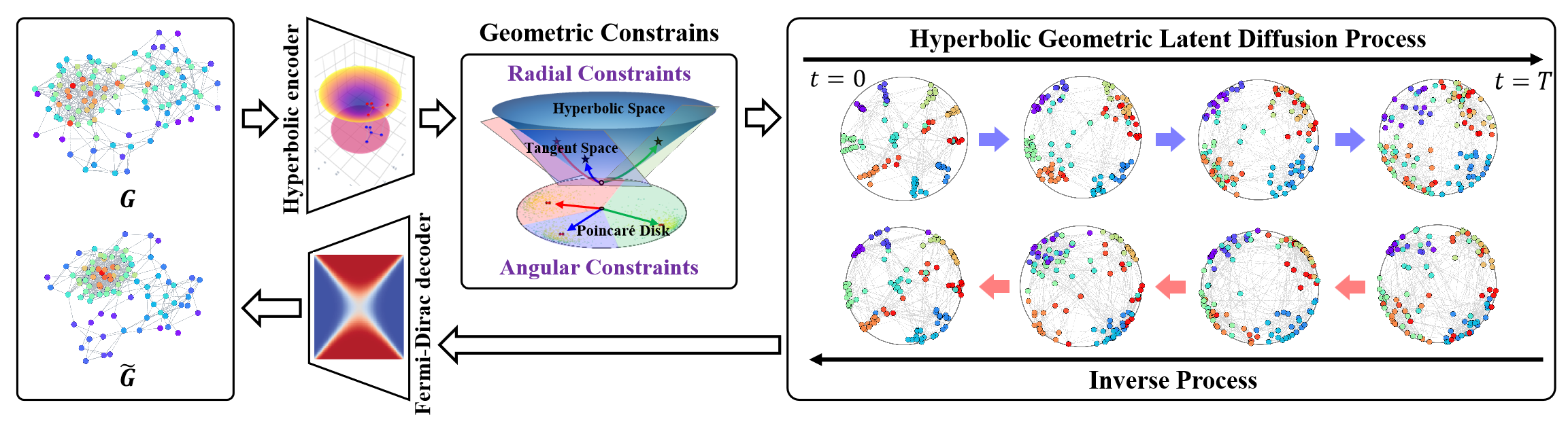
In this context, the HypDiff framework represents an advanced method for generating hyperbolic Gaussian noise, effectively resolving the issue of additive perturbations in Gaussian distributions within hyperbolic space. The authors of the framework introduced geometric constraints based on angular similarity, applied in the process of anisotropic diffusion to preserve the local structure of graphs.

The original visualization of the framework is provided below.

In the previous article, we began implementing the proposed approaches in MQL5. However, the scope of work is quite extensive. We were only able to cover the implementation blocks on the OpenCL program side. In this article, we will continue the work we started and bring the HypDiff framework implementation to a logical conclusion. Nevertheless, in our implementation, we will introduce certain deviations from the original algorithm, which we will discuss throughout the algorithm development process.

1. Data Projection into Hyperbolic Space

Our work on the OpenCL program side began with the development of kernels for the feed-forward and backpropagation passes of projecting the original data into hyperbolic space (HyperProjection and HyperProjectionGrad, respectively). Likewise, we will begin implementing the HypDiff framework on the main program side by constructing the algorithms for this functionality. To do this, we will create a new class, CNeuronHyperProjection, the structure of which is presented below.

class CNeuronHyperProjection   :  public CNeuronBaseOCL
  {
protected:
   uint              iWindow;
   uint              iUnits;
   //---
   virtual bool      feedForward(CNeuronBaseOCL *NeuronOCL);
   virtual bool      calcInputGradients(CNeuronBaseOCL *prevLayer);
   virtual bool      updateInputWeights(CNeuronBaseOCL *NeuronOCL)   { return true; }

public:
                     CNeuronHyperProjection(void) : iWindow(-1), iUnits(-1) {};
                    ~CNeuronHyperProjection(void) {};
   //---
   virtual bool      Init(uint numOutputs, uint myIndex, COpenCLMy *open_cl, 
                          uint window, uint units_count, 
                          ENUM_OPTIMIZATION optimization_type, uint batch);
   //---
   virtual int       Type(void)   const   {  return defNeuronHyperProjection;   }
   //--- methods for working with files
   virtual bool      Save(int const file_handle);
   virtual bool      Load(int const file_handle);
  };

In the presented structure, we see the declaration of two internal variables used to store constants that define the architecture of the object, along with the familiar set of overridable methods. However, note that the model parameter update method updateInputWeights is implemented as a positive "stub". This is done on purpose. The feed-forward and backpropagation projection kernels we developed implement an explicitly defined algorithm that does not include any trainable parameters. Nonetheless, the presence of a parameter update method is required for the correct functioning of our model. Therefore, we are compelled to override the specified method to always return a positive result.

The absence of newly declared internal objects allows us to leave the class constructor and destructor empty. The initialization of inherited objects and internal variables is handled within the Init method.

The initialization method's algorithm is fairly straightforward. As usual, its parameters include the core constants necessary to unambiguously identify the architecture of the object being created.

bool CNeuronHyperProjection::Init(uint numOutputs, uint myIndex, COpenCLMy *open_cl, 
                                  uint window, uint units_count, 
                                  ENUM_OPTIMIZATION optimization_type, uint batch)
  {
   if(!CNeuronBaseOCL::Init(numOutputs, myIndex, open_cl, (window + 1)*units_count, optimization_type, batch))
      return false;
   iWindow = window;
   iUnits = units_count;
//---
   return true;
  }

Within the body of the method, we immediately call the identically-named method of the parent class, passing it the relevant portion of the received parameters. As you know, the parent class already implements the logic for validating these parameters and initializing inherited objects. All we need to do is check the logical result of the parent method execution. After that, we save the architectural constants received from the external program into the internal variables.

That's it. We haven't declared any new internal objects, and the inherited ones are initialized in the parent class method. All that remains is to return the result of the operations to the calling program and exit the method.

As for the feed-forward and backpropagation methods of this class, I suggest you review them on your own. Both are simple "wrappers" that call the corresponding kernels of the OpenCL program. Similar methods have been described many times throughout our article series. I believe their implementation logic will be clear to you. The full code of this class and all its methods can be found in the attachment.

2. Projection onto Tangent Planes

After projecting the original data into hyperbolic space, the HypDiff framework calls for the construction of an encoder for generating hyperbolic node embeddings. We plan to implement this functionality using existing components from our library. The resulting embeddings are projected onto tangent planes corresponding to k centroids. We have already implemented the projection algorithms for tangent mapping and the corresponding gradient back-distribution on the OpenCL side via the LogMap and LogMapGrad kernels, respectively. However, the question of centroids remains unresolved.

It should be noted that the authors of the HypDiff framework defined centroids from the training dataset during the data preparation stage. Unfortunately, such an approach is not suitable for our purposes. And it's not just its labor intensity. This method is not suitable for analysis in the context of the dynamic financial markets. In technical analysis of price movements, emerging patterns often take precedence over specific price values. For similar market situations observed over different time intervals, different centroids may be relevant. From this, we conclude that it is necessary to create a dynamic model for adapting or generating centroids and their parameters. In our implementation, we decided to pursue a centroid generation model based on embeddings of the original data. As a result, we chose to combine the processes of centroid generation and data projection onto the corresponding tangent planes within a single class: CNeuronHyperboloids. Its structure is presented below.

class CNeuronHyperboloids  :  public CNeuronBaseOCL
  {
protected:
   uint              iWindows;
   uint              iUnits;
   uint              iCentroids;
   //---
   CLayer            cHyperCentroids;
   CLayer            cHyperCurvatures;
   //---
   int               iProducts;
   int               iDistances;
   int               iNormes;
   //---
   virtual bool      LogMap(CNeuronBaseOCL *featers, CNeuronBaseOCL *centroids, 
                            CNeuronBaseOCL *curvatures, CNeuronBaseOCL *outputs);
   virtual bool      LogMapGrad(CNeuronBaseOCL *featers, CNeuronBaseOCL *centroids, 
                                CNeuronBaseOCL *curvatures, CNeuronBaseOCL *outputs);
   //---
   virtual bool      feedForward(CNeuronBaseOCL *NeuronOCL);
   virtual bool      calcInputGradients(CNeuronBaseOCL *prevLayer);
   virtual bool      updateInputWeights(CNeuronBaseOCL *NeuronOCL);

public:
                     CNeuronHyperboloids(void) : iWindows(0), iUnits(0), iCentroids(0), 
                                                 iProducts(-1), iDistances(-1), iNormes(-1) {};
                    ~CNeuronHyperboloids(void) {};
   //---
   virtual bool      Init(uint numOutputs, uint myIndex, COpenCLMy *open_cl, 
                          uint window, uint units_count, uint centroids, 
                          ENUM_OPTIMIZATION optimization_type, uint batch);
   //---
   virtual int       Type(void)   const   {  return defNeuronHyperboloids;   }
   //--- methods for working with files
   virtual bool      Save(int const file_handle);
   virtual bool      Load(int const file_handle);
   //---
   virtual bool      WeightsUpdate(CNeuronBaseOCL *source, float tau);
   virtual void      SetOpenCL(COpenCLMy *obj);
   virtual void      TrainMode(bool flag);
  };

In the presented structure of the new class, we can observe the declaration of two dynamic arrays and six variables, divided into two groups.

The dynamic arrays are intended to store pointers to the neural layer objects of two nested models. Indeed, in our implementation, we decided to split the functionality for generating centroid parameters into two separate models. The first model is responsible for generating the coordinates of centroids in hyperbolic space. The second returns the curvature parameters of the space at the corresponding points.

The grouping of internal variables also follows a logical explanation. One group contains the architectural parameters of the object being created, which we receive from the external program. The second group consists of variables that store pointers to buffers used for intermediate values, which are created exclusively within the OpenCL context, without copying data into the system's main memory.

All internal objects are declared statically, which allows us to leave the class constructor and destructor empty. Initialization of all inherited and declared objects is implemented in the Init method.

bool CNeuronHyperboloids::Init(uint numOutputs, uint myIndex, COpenCLMy *open_cl, 
                               uint window, uint units_count, uint centroids,
                               ENUM_OPTIMIZATION optimization_type, uint batch)
  {
   if(!CNeuronBaseOCL::Init(numOutputs, myIndex, open_cl, window*units_count*centroids, optimization_type, batch))
      return false;

As usual, the method parameters include a number of constants that unambiguously define the architecture of the object being created. These include:

• units_count — the number of elements in the sequence being analyzed;
• window — the size of the embedding vector for a single element in the analyzed sequence;
• centroids — the number of centroids generated by the model for comprehensive analysis of the original data.

In the method body, following our established approach, we call the identically-named method of the parent class to initialize the inherited objects and variables. It is worth noting here that, unlike in the original HypDiff algorithm, our implementation does not assign individual elements of the input sequence to specific centroids. Instead, to provide the model with the maximum amount of information, we generate projections of the entire sequence onto all tangent planes. Naturally, this increases the size of the resulting tensor in proportion to the number of generated centroids. Therefore, when calling the parent class initialization method, we specify the product of all three externally supplied constants as the size of the created layer.

Once the parent method completes successfully, which will be indicated by its boolean logical return value, we save the received constants in the internal variables.

   iWindows = window;
   iUnits = units_count;
   iCentroids = centroids;

In the next step, we will prepare our dynamic arrays to store pointers to the objects of the centroid parameter generation models.

   cHyperCentroids.Clear();
   cHyperCurvatures.Clear();
   cHyperCentroids.SetOpenCL(OpenCL);
   cHyperCurvatures.SetOpenCL(OpenCL);

Then we proceed directly to the initialization of the model objects. First, we initialize the model responsible for generating the centroid coordinates.

Here, we aim to construct a linear model that, after analyzing the input data, returns a batch of coordinates for the relevant centroids. However, the use of fully connected layers for this purpose leads to the creation of a large number of trainable parameters and increased computational load. The use of convolutional layers allows us to reduce both the number of trainable parameters and the volume of computations. Moreover, applying convolutional layers to individual univariate sequences appears to be a logical approach. To implement this, we first need to transpose the input data accordingly.

   CNeuronTransposeOCL *transp = new CNeuronTransposeOCL();
   if(!transp ||
      !transp.Init(0, 0, OpenCL, iUnits, iWindows, optimization, iBatch) ||
      !cHyperCentroids.Add(transp))
     {
      delete transp;
      return false;
     }
   transp.SetActivationFunction(None);

Next, we add a convolutional layer to reduce the dimensionality of the univariate sequences.

   CNeuronConvOCL *conv = new CNeuronConvOCL();
   if(!conv ||
      !conv.Init(0, 1, OpenCL, iUnits, iUnits, iCentroids, iWindows, 1, optimization, iBatch) ||
      !cHyperCentroids.Add(conv))
     {
      delete conv;
      return false;
     }
   conv.SetActivationFunction(TANH);

In this layer, we use a shared set of parameters across all univariate sequences. At the output of the layer, we apply the hyperbolic tangent function as an activation function to introduce non-linearity.

We then add another convolutional layer, without an activation function but with distinct trainable parameters for each univariate sequence.

   conv = new CNeuronConvOCL();
   if(!conv ||
      !conv.Init(0, 2, OpenCL, iCentroids, iCentroids, iCentroids, 1, iWindows, optimization, iBatch) ||
      !cHyperCentroids.Add(conv))
     {
      delete conv;
      return false;
     }
   conv.SetActivationFunction(None);

As a result, the two sequential convolutional layers effectively form a unique MLP for each univariate series in the input sequence. Each such MLP generates one coordinate for the required number of centroids. In other words, we have built an MLP for each dimension of the coordinate space, and together, they generate the full set of coordinates for the specified number of centroids.

Now, we only need to return the generated centroid coordinates to their original representation. To achieve this, we add another data transposition layer.

   transp = new CNeuronTransposeOCL();
   if(!transp ||
      !transp.Init(0, 3, OpenCL, iWindows, iCentroids, optimization, iBatch) ||
      !cHyperCentroids.Add(transp))
     {
      delete transp;
      return false;
     }
   transp.SetActivationFunction((ENUM_ACTIVATION)conv.Activation());

Next, we move on to constructing the objects for the second model, which will determine the curvature parameters of the hyperbolic space at the centroid locations. The curvature parameters will be derived based on the generated centroid coordinates. It is reasonable to assume that the curvature parameter depends solely on the specific coordinates. Because we expect the model to form an internal representation of the hyperbolic space during training and reflect this in its learned parameters. Therefore, in the curvature parameter model, we no longer use transposition layers. Instead, we simply create a unique MLP for each centroid, composed of two consecutive convolutional layers.

   conv = new CNeuronConvOCL();
   if(!conv ||
      !conv.Init(0, 4, OpenCL, iWindows, iWindows, iWindows, iCentroids, 1, optimization, iBatch) ||
      !cHyperCurvatures.Add(conv))
     {
      delete conv;
      return false;
     }
   conv.SetActivationFunction(TANH);
//---
   conv = new CNeuronConvOCL();
   if(!conv ||
      !conv.Init(0, 5, OpenCL, iWindows, iWindows, 1, 1, iCentroids, optimization, iBatch) ||
      !cHyperCurvatures.Add(conv))
     {
      delete conv;
      return false;
     }
   conv.SetActivationFunction(None);

Here we also use the hyperbolic tangent function to introduce non-linearity between the layers of the model.

At this stage, we complete the initialization of the model objects responsible for generating the centroid parameters. What remains is to prepare the objects required to support the kernels for projecting data onto tangent planes and distributing gradient errors. Here, I'd like to remind you that during the development of the aforementioned kernels, we discussed the creation of temporary buffers to store intermediate results. These are three data buffers, each containing one element per "Centroid — Sequence Element" pair.

These buffers are used solely to transfer information from the feed-forward pass kernel to the gradient distribution kernel. Accordingly, their creation is justified only within the OpenCL context. In other words, allocating these buffers in system memory and copying data between the OpenCL context and main memory would be redundant. Likewise, there is no need to save these buffers when storing model parameters, as they are updated during each forward pass. Therefore, on the side of the main program, we only declare variables to hold pointers to these data buffers.

However, we still need to create the buffers within the OpenCL context. To do this, we first determine the required size of the data buffers. As mentioned earlier, all three buffers share the same size.

   uint size = iCentroids * iUnits * sizeof(float);
   iProducts = OpenCL.AddBuffer(size, CL_MEM_READ_WRITE);
   if(iProducts < 0)
      return false;
   iDistances = OpenCL.AddBuffer(size, CL_MEM_READ_WRITE);
   if(iDistances < 0)
      return false;
   iNormes = OpenCL.AddBuffer(size, CL_MEM_READ_WRITE);
   if(iNormes < 0)
      return false;
//---
   return true;
  }

Next, we create the data buffers in OpenCL memory and store the resulting pointers in the appropriate variables. As always, we check the validity of the received pointer.

Once all objects have been initialized, we return the logical result of the operation to the caller and complete the method execution.

The next stage of our work is to develop the feed-forward pass algorithms for our CNeuronHyperboloids class. It should be mentioned here that the LogMap and LogMapGrad methods are wrappers for calling the corresponding OpenCL kernels. We will leave those for you to explore independently.

Let's look at the feedForward method. In the parameters of this method, we receive a pointer to the neural layer object, which contains the tensor of the original data.

bool CNeuronHyperboloids::feedForward(CNeuronBaseOCL *NeuronOCL)
  {
   CNeuronBaseOCL *prev = NeuronOCL;
   CNeuronBaseOCL *centroids = NULL;
   CNeuronBaseOCL *curvatures = NULL;

And in the body of the method, we first do a little preparatory work: we will declare local variables for temporary storage of pointers to objects of internal neural layers. One of these is assigned the received pointer to the input data object. The other two will remain empty for now.

Note that at this point, we do not check the validity of the received input data pointer. The method does not directly access the data buffers of this object during its execution. Therefore, such a check would be unnecessary

Next, we proceed to generate the centroid coordinates for the current set of input data. To do this, we loop over the objects of the corresponding internal model.

//--- Centroids
   for(int i = 0; i < cHyperCentroids.Total(); i++)
     {
      centroids = cHyperCentroids[i];
      if(!centroids ||
         !centroids.FeedForward(prev))
         return false;
      prev = centroids;
     }

Within the loop body, we sequentially retrieve pointers to the neural layer objects and check their validity. We then call the feedForward method of the retrieved internal object, passing to it the appropriate input data pointer from the corresponding local variable. Upon successful execution of the internal layer’s forward pass, this object becomes the source of input data for the next layer in the model. Consequently, we store its pointer in the local input data variable.

Note that this local variable initially held the pointer to the input data object received from the external program. Therefore, during the first iteration of our loop, we used it as the input data. This means that the validity od the external data pointer is checked in the internal model layer's feed-forward method. Thus, all control points are enforced, and the data flow from the input object is preserved.

We organize a similar loop to determine the curvature parameters of the hyperbolic space at the centroid points. Note that after completing the iterations of the previous loop, the local variables prev and centroids both point to the final layer object of the centroid coordinate generation model. Since the curvature parameters are to be determined based on the centroid coordinates, we can confidently proceed using the prev variable.

//--- Curvatures
   for(int i = 0; i < cHyperCurvatures.Total(); i++)
     {
      curvatures = cHyperCurvatures[i];
      if(!curvatures ||
         !curvatures.FeedForward(prev))
         return false;
      prev = curvatures;
     }

Once all necessary centroid parameters are successfully obtained, we can perform the projection of the input data onto the corresponding tangent planes. To achieve this, we invoke the wrapper method for the LogMap kernel introduced in the previous article.

   if(!LogMap(NeuronOCL, centroids, curvatures, AsObject()))
      return false;
//---
   return true;
  }

Note that we pass the pointer to the current object as the result-receiving entity. This allows us to save the operation results within the interface buffers of our class, which will be accessed by subsequent neural layers of the model.

We now just need to return the logical result of the operations to the caller and complete the feed-forward pass method.

After implementing feed-forward methods, we move on to developing the backpropagation algorithms. Here, I propose we focus on the calcInputGradients method, which handles the gradient distribution. The updateInputWeights method will be left for your independent review.

As usual, the calcInputGradients method receives a pointer to the preceding layer's object, into whose buffer we are to transmit the error gradient calculated based on the influence of the input data on the model's final output.

bool CNeuronHyperboloids::calcInputGradients(CNeuronBaseOCL *prevLayer)
  {
   if(!prevLayer)
      return false;

This time we immediately check the correctness of the received pointer. Because if you receive an incorrect pointer, all further operations immediately lose their meaning.

Just as in the feed-forward pass, we declare local variables to temporarily store pointers to internal model objects. However, this time we will immediately extract the pointers to the last layers of the internal models.  

   CObject *next = NULL;
   CNeuronBaseOCL *centroids = cHyperCentroids[-1];
   CNeuronBaseOCL *curvatures = cHyperCurvatures[-1];

After that, we call the wrapper method of the gradient distribution kernel through the operations of projection of the original data onto the tangent planes.

   if(!LogMapGrad(prevLayer, centroids, curvatures, AsObject()))
      return false;

Then we distribute the error gradient according to the internal model for determining the curvature of hyperspace at the centroid points, creating a cycle of reverse enumeration of the neural layers of the model.

//--- Curvatures
   for(int i = cHyperCurvatures.Total() - 2; i >= 0; i--)
     {
      next = curvatures;
      curvatures = cHyperCurvatures[i];
      if(!curvatures ||
         !curvatures.calcHiddenGradients(next))
         return false;
     }

And then we need to pass the error gradient from the curvature determination model to the centroid coordinate generation model. But here we notice that the buffer of the last layer of the centroid coordinate generation model already contains an error gradient from the operations of projecting data onto tangent planes. And we want to retain these values. In such cases, we resort to substituting pointers to data buffers. First, we save the current pointer to the error gradient buffer of the last layer of the centroid coordinate generation model in a local variable and, if necessary, adjust the values by the derivative of the activation function of the neural layer.

   CBufferFloat *temp = centroids.getGradient();
   if(centroids.Activation()!=None)
      if(!DeActivation(centroids.getOutput(),temp,temp,centroids.Activation()))
        return false;
   if(!centroids.SetGradient(centroids.getPrevOutput(), false) ||
      !centroids.calcHiddenGradients(curvatures.AsObject()) ||
      !SumAndNormilize(temp, centroids.getGradient(), temp, iWindows, false, 0, 0, 0, 1) ||
      !centroids.SetGradient(temp, false)
     )
      return false;

Then we temporarily replace it with an unused buffer of the appropriate size. We call the error gradient distribution method for the last layer of the centroid coordinate generation model, passing it the first layer of the hyperspace curvature determination model at the centroid points as a subsequent object. We sum the values of the two data buffers and return their pointers to their original state. Remember to control the execution of all operations.

Now, that we have the total error gradient in the last layer's buffer of the model for determining centroid coordinates, we can create a loop for backward iteration through the neural layers of the model. In this loop, we organize the distribution of the error gradient between the layers of the model depending on their contribution to the final result.

//--- Centroids
   for(int i = cHyperCentroids.Total() - 2; i >= 0; i--)
     {
      next = centroids;
      centroids = cHyperCentroids[i];
      if(!centroids ||
         !centroids.calcHiddenGradients(next))
         return false;
     }

Finally, we propagate the accumulated error gradient to the input data level. But here we again face the question of preserving the previously accumulated error gradient. So, we substitute data buffers for the input data object.

   temp = prevLayer.getGradient();
   if(prevLayer.Activation()!=None)
      if(!DeActivation(prevLayer.getOutput(),temp,temp,prevLayer.Activation()))
        return false;
   if(!prevLayer.SetGradient(prevLayer.getPrevOutput(), false) ||
      !prevLayer.calcHiddenGradients(centroids.AsObject()) ||
      !SumAndNormilize(temp, prevLayer.getGradient(), temp, iWindows, false, 0, 0, 0, 1) ||
      !prevLayer.SetGradient(temp, false)
     )
      return false;
//---
   return true;
  }

Then we return the result of the operations to the caller and exit the method.

This concludes our review of the implementation of methods on our new class CNeuronHyperboloids. You can find the complete code of this class and all its methods in the attachment.

3. Building the HypDiff Framework

We have completed the development of the individual new components of the HypDiff framework and have now reached the stage of constructing a unified object representing the top-level implementation of the framework. To achieve this, we create a new class CNeuronHypDiff with the structure presented below.

class CNeuronHypDiff :  public CNeuronRMAT
  {
public:
                     CNeuronHypDiff(void) {};
                    ~CNeuronHypDiff(void) {};
   //---
   virtual bool      Init(uint numOutputs, uint myIndex, COpenCLMy *open_cl,
                          uint window, uint window_key, uint units_count,
                          uint heads, uint layers, uint centroids,
                          ENUM_OPTIMIZATION optimization_type, uint batch);
   //---
   virtual int       Type(void) override   const   {  return defNeuronHypDiff; }
   //---
   virtual uint      GetWindow(void) const override
     {
      CNeuronRMAT* neuron = cLayers[1];
      return (!neuron ? 0 : neuron.GetWindow() - 1);
     }
   virtual uint      GetUnits(void) const override
     {
      CNeuronRMAT* neuron = cLayers[1];
      return (!neuron ? 0 : neuron.GetUnits());
     }
  };

As can be seen from the structure of the new class, its core functionality is inherited from the CNeuronRMAT object. This base object provides functionality for organizing the operation of a small linear model, which is entirely sufficient for implementing the HypDiff framework. Therefore, at this stage, it is enough to override the object initialization method, specifying the correct architecture for the embedded model. All other processes are already covered by the parent class methods.

Within the parameters of the initialization method, we receive the primary constants that allow for the unambiguous interpretation of the architecture of the object being created.

bool CNeuronHypDiff::Init(uint numOutputs, uint myIndex, COpenCLMy *open_cl, 
                          uint window, uint window_key, uint units_count, 
                          uint heads, uint layers, uint centroids, 
                          ENUM_OPTIMIZATION optimization_type, uint batch)
  {
   if(!CNeuronBaseOCL::Init(numOutputs, myIndex, open_cl, window * units_count, optimization_type, batch))
      return false;

Inside the method body, we immediately call the corresponding method of the base neural layer object, within which the initialization of core interfaces is implemented. We intentionally avoid calling the initialization method of the direct parent class at this stage, as the architecture of the embedded model we are creating differs significantly.

Next, we prepare the inherited dynamic array to store pointers to the internal objects.

   cLayers.Clear();
   cLayers.SetOpenCL(OpenCL);
   int layer = 0;

Then we proceed directly to constructing the internal architecture of the HypDiff framework.

The input data passed into the model is first projected into hyperbolic space. For this purpose, we add an instance of the previously created CNeuronHyperProjection class.

//--- Projection
   CNeuronHyperProjection *lorenz = new CNeuronHyperProjection();
   if(!lorenz ||
      !lorenz.Init(0, layer, OpenCL, window, units_count, optimization, iBatch) ||
      !cLayers.Add(lorenz))
     {
      delete lorenz;
      return false;
     }
   layer++;

The HypDiff framework then requires a hyperbolic encoder designed to generate embeddings for the nodes of the analyzed graph. The authors of the original framework used graph neural models combined with convolutional layers for this stage. In our implementation, we will replace the graph neural networks with a Transformer that uses relative positional encoding.

//--- Encoder
   CNeuronRMAT *rmat = new CNeuronRMAT();
   if(!rmat ||
      !rmat.Init(0, layer, OpenCL, window + 1, window_key, units_count, heads, layers, optimization, iBatch) ||
      !cLayers.Add(rmat))
     {
      delete rmat;
      return false;
     }
   layer++;
//---
   CNeuronConvOCL *conv = new CNeuronConvOCL();
   if(!conv ||
      !conv.Init(0, layer, OpenCL, window + 1, window + 1, 2 * window, units_count, 1, optimization, iBatch) ||
      !cLayers.Add(conv))
     {
      delete conv;
      return false;
     }
   layer++;
   conv.SetActivationFunction(TANH);
//---
   conv = new CNeuronConvOCL();
   if(!conv ||
      !conv.Init(0, layer, OpenCL, 2 * window, 2 * window, 3, units_count, 1, optimization, iBatch) ||
      !cLayers.Add(conv))
     {
      delete conv;
      return false;
     }
   layer++;

It is important to note that when projecting the resulting embeddings onto the tangent planes, we significantly increase the volume of processed information by performing projections onto all tangent planes using the full body of data. To partially mitigate the negative impact of this approach, we reduce the dimensionality of each node's embedding.

The resulting data embeddings must then be projected onto the tangent planes of the centroids. The functionality for centroid generation and projection of input data onto the corresponding tangent spaces has already been implemented in the CNeuronHyperboloids class. At this point, it is sufficient to add an instance of that object into our linear model.

//--- LogMap projecction
   CNeuronHyperboloids *logmap = new CNeuronHyperboloids();
   if(!logmap ||
      !logmap.Init(0, layer, OpenCL, 3, units_count, centroids, optimization, iBatch) ||
      !cLayers.Add(logmap))
     {
      delete logmap;
      return false;
     }
   layer++;

At the output, we obtain projections of the input data across multiple planes. These can now be processed using the directed diffusion algorithm, originally developed for Euclidean models. In our implementation, we used the CNeuronDiffusion object for this purpose.

//--- Diffusion model
  CNeuronDiffusion *diff = new CNeuronDiffusion();
  if(!diff ||
     !diff.Init(0, layer, OpenCL, 3, window_key, heads, units_count*centroids, 2, layers, optimization, iBatch) ||
     !cLayers.Add(diff))
    {
     delete diff;
     return false;
    }
  layer++;

One key aspect to note here is that we did not consolidate the various projections of a single sequence element into a single entity. On the contrary, our diffusion model treats each projection as an independent object. In doing so, we enable the model to learn to correlate different projections of the same sequence and to form a volumetric representation of the underlying data.

Another implicit detail worth noting is the injection of noise. We chose not to complicate the model by trying to match noise across projections of the same sequence element. The very act of adding noise implies a form of blurring of the original inputs within some neighborhood. By introducing varied noise across different projections, we achieve a volumetric blur.

At the output of the diffusion model, we expect to obtain a denoised representation of the input data across multiple projections. And here is where our implementation diverges most significantly from the original HypDiff framework. In the original, the authors performed an inverse projection back into hyperbolic space and used a Fermi-Dirac decoder to reconstruct the original graph representation. Our goal is to obtain an informative latent representation of the input data that can be passed to an Actor model for learning a profitable policy for our agent's behavior. Therefore, instead of decoding, we apply a dependency-based pooling layer to derive a unified representation for each sequence element.

//--- Pooling
   CNeuronMHAttentionPooling *pooling = new CNeuronMHAttentionPooling();
   if(!pooling ||
      !pooling.Init(0, layer, OpenCL, 3, units_count, centroids, optimization, iBatch) ||
      !cLayers.Add(pooling))
     {
      delete pooling;
      return false;
     }
   layer++;

Change the size of the result tensor to the level of the input data.

//--- Resize to source size
   conv = new CNeuronConvOCL();
   if(!conv ||
      !conv.Init(0, layer, OpenCL, 3, 3, window, units_count, 1, optimization, iBatch) ||
      !cLayers.Add(conv))
     {
      delete conv;
      return false;
     }

Now we just need to replace the pointers of the interface data buffers with the corresponding buffers of the last layer of our model. And then we complete the work of the initialization method of our class.

//---
   if(!SetOutput(conv.getOutput(), true) ||
      !SetGradient(conv.getGradient(), true))
      return false;
//---
   return true;
  }

This concludes the implementation of our own interpretation of the HypDiff framework using MQL5. The full source code for all classes and methods discussed in this article is available in the attachment. You will also find the code for environment interaction and model training programs, which were carried over unchanged from previous works.

A few final remarks about the architecture of the trainable models. The Actor and Critic model architectures remain unchanged. However, we made slight modifications to the environment state encoder model. The input data to this model, as before, undergoes initial preprocessing via a batch normalization layer.

bool CreateEncoderDescriptions(CArrayObj *&encoder)
  {
//---
   CLayerDescription *descr;
//---
   if(!encoder)
     {
      encoder = new CArrayObj();
      if(!encoder)
         return false;
     }
//--- Encoder
   encoder.Clear();
//--- Input layer
   if(!(descr = new CLayerDescription()))
      return false;
   descr.type = defNeuronBaseOCL;
   int prev_count = descr.count = (HistoryBars * BarDescr);
   descr.activation = None;
   descr.optimization = ADAM;
   if(!encoder.Add(descr))
     {
      delete descr;
      return false;
     }
//--- layer 1
   if(!(descr = new CLayerDescription()))
      return false;
   descr.type = defNeuronBatchNormOCL;
   descr.count = prev_count;
   descr.batch = 1e4;
   descr.activation = None;
   descr.optimization = ADAM;
   if(!encoder.Add(descr))
     {
      delete descr;
      return false;
     }

After that they are immediately passed into our hyperbolic latent diffusion model.

//--- layer 2
   if(!(descr = new CLayerDescription()))
      return false;
   descr.type = defNeuronHypDiff;
   descr.count = HistoryBars;
   descr.window = BarDescr;
   descr.window_out = BarDescr;
   descr.layers=2;
   descr.step=10;                                        // centroids
   {
      int temp[] = {4};                                  // Heads
      if(ArrayCopy(descr.heads, temp) < (int)temp.Size())
         return false;
   }
   descr.batch = 1e4;
   descr.activation = None;
   descr.optimization = ADAM;
   if(!encoder.Add(descr))
     {
      delete descr;
      return false;
     }

The above described algorithm of the hyperbolic latent diffusion model is a rather complex and comprehensive process. Therefore, we excluded further data processing. We used only one fully connected layer to reduce the data to the required tensor size, which is input into the Actor model.

//--- layer 3
   if(!(descr = new CLayerDescription()))
      return false;
   descr.type = defNeuronBaseOCL;
   descr.count = LatentCount;
   descr.activation = None;
   descr.optimization = ADAM;
   if(!encoder.Add(descr))
     {
      delete descr;
      return false;
     }
//---
   return true;
  }

At this point, we conclude the implementation of the HypDiff framework approaches and move on to the most anticipated stage — the practical evaluation of results on real historical data.

4. Testing

We have implemented the HypDiff framework using MQL5 and now proceed to the final phase — training the models and evaluating the resulting Actor policy. We follow the training algorithm described in previous works, and we simultaneously train three models: the State Encoder, Actor, and Critic. The Encoder analyzes the market environment. The Actor makes trading decisions based on the learned policy. The Critic evaluates the Actor's actions and guides policy refinement.

Training is conducted using real historical data for the entire year of 2023 on the EURUSD instrument with the H1 timeframe. All indicator parameters were set to their default values.

The training process is iterative and includes regular updates to the training dataset.

To verify the effectiveness of the trained policy, we use historical data for the first quarter of 2024. The test results are presented below.

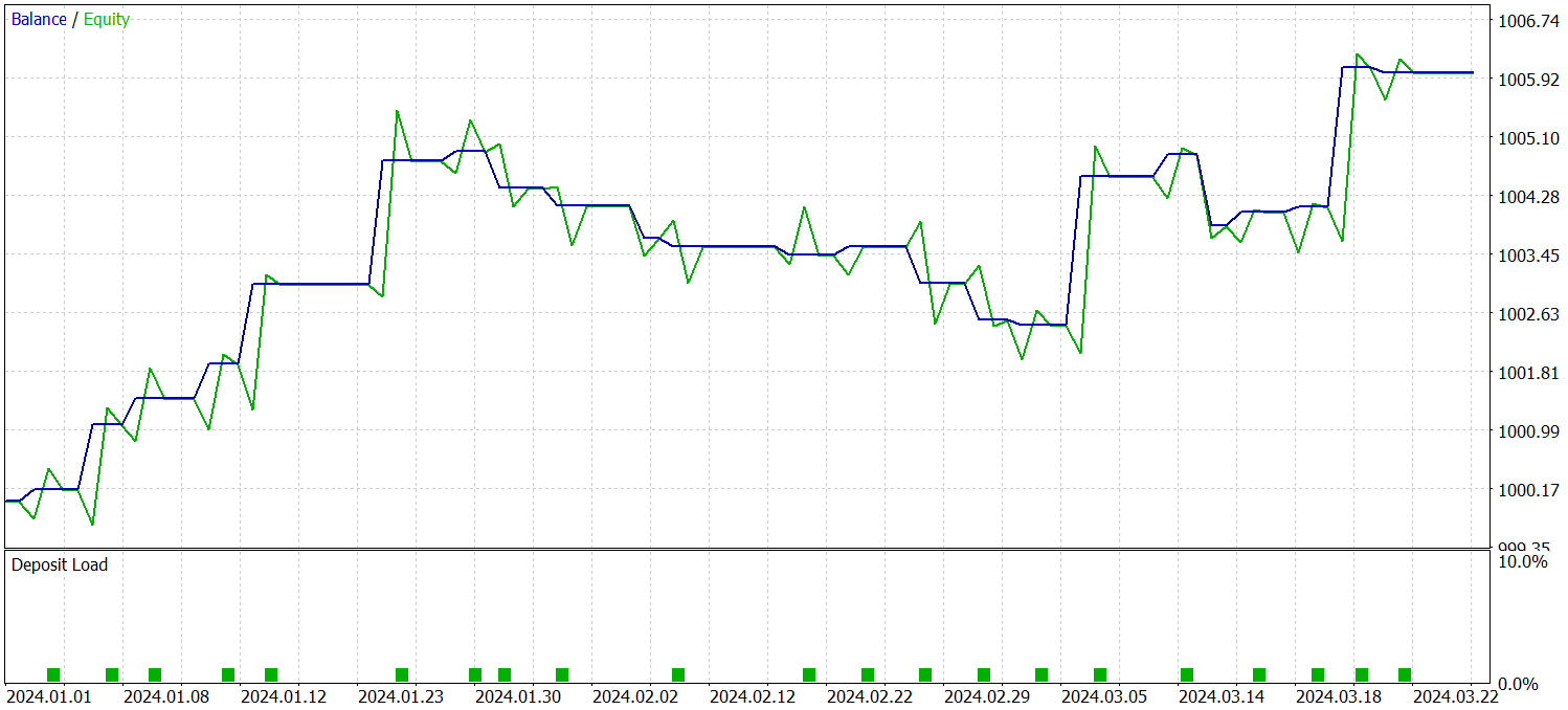
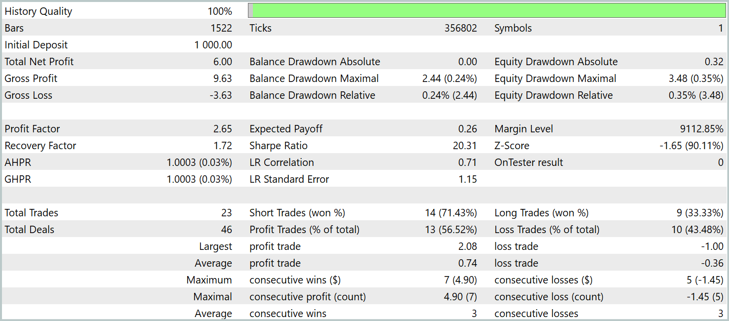
As the data shows, the model successfully generated a profit during the testing period. A total of 23 trades were executed over the course of three months, which is a relatively small number. Over 56% of the trades were closed profitably. Both the maximum and average profit per trade being approximately twice as large as their loss counterparts.

However, a more compelling insight comes from a detailed breakdown of the trades. Out of the three testing months, the model was profitable in only two. February was entirely unprofitable. In January 2024, 7 out of 8 trades were profitable — the only loss occurred on the final trade of the month. This outcome supports the previously stated hypothesis about the limited representativeness of a one-year training sample beyond the model's first month of deployment.

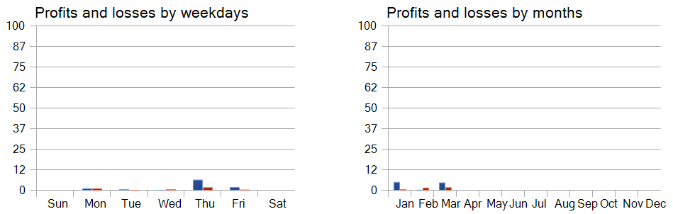
A performance analysis across the days of the week also reveals a distinct preference for trading on Thursdays and Fridays.

Conclusion

The application of hyperbolic geometry helps address challenges arising from the inherent conflict between the discrete nature of graph-structured data and the continuous nature of diffusion models. The HypDiff framework introduces an enhanced method for generating hyperbolic Gaussian noise, resolving issues related to additive inconsistencies of Gaussian distributions in hyperbolic space. To preserve local structure during anisotropic diffusion, geometric constraints based on angular similarity are imposed.

In the practical part of our work, we implemented our interpretation of these methods using MQL5 We trained the models on real historical data using the proposed techniques. We also evaluated the Actor's learned policy on data outside the training set. The results demonstrate the potential of the proposed methods and point toward possible directions for improving model performance.

References

• Hyperbolic Geometric Latent Diffusion Model for Graph Generation
• Other articles from this series

Programs used in the article

#	Name	Type	Description
1	Research.mq5	Expert Advisor	EA for collecting examples
2	ResearchRealORL.mq5	Expert Advisor	EA for collecting examples using the Real-ORL method
3	Study.mq5	Expert Advisor	Model training EA
4	Test.mq5	Expert Advisor	Model testing EA
5	Trajectory.mqh	Class library	System state description structure
6	NeuroNet.mqh	Class library	A library of classes for creating a neural network
7	NeuroNet.cl	Library	OpenCL program code library