From Novice to Expert: Creating a Liquidity Zone Indicator

Contents:

1. Introduction
2. Reviewing the concept
3. Implementation
4. Test
5. Conclusion
6. Key Lessons
7. Attachments

Introduction

In our previous article, we embarked on a deep research journey to uncover the potential ratios between liquidity zones and their subsequent breakout ranges. Statistically, the most consistent conceptual ratio that emerged was 1:3 (liquidity zone depth to breakout/impulse range).

Now that we've identified this key value, the next logical step is clear: turning insight into actionable edge. Traders everywhere want to know—how exactly does this 1:3 ratio become practically useful? The answer lies in strategy development.

Today, we anchor our discussion on building a custom indicator that brings these ratios to life, transforming theoretical observations into real-time, practical signals on your charts. Below, I'll first review the core concept to ensure it clicks fully before we dive into the implementation phase.

Reviewing the concept

Liquidity zones represent periods of market consolidation—distinct ranges where price oscillates between two well-defined levels over time. For clarity, let’s use Price A and Price B as conceptual reference points for the boundaries of the base rather than fixed or absolute price levels. In a typical bullish setup, Price A represents the low of the base while Price B marks the high of the base; price fluctuates between these two levels during the consolidation phase. In bearish scenarios, this structure is simply mirrored (with Price A as the high and Price Bas the low of the base). Although the market appears balanced during these pauses, institutional participants are actively accumulating or distributing positions, with liquidity deliberately building around the range extremes.

Eventually, price exits this equilibrium through an impulsive breakout. In bullish conditions, this breakout occurs above Price B(the high of the base), while in bearish conditions it occurs below Price A (the low of the base). The breakout establishes a new reference level, which we denote as Price C—the high formed by the impulsive rally in bullish cases, or the low formed by the impulsive sell-off in bearish cases. These moves are rarely accidental; they are typically driven by the absorption of resting liquidity, including stop-loss orders positioned beyond the range, breakout orders from retail participants, and trapped positions on the wrong side of consolidation.

In high-probability environments—whether continuation scenarios following a liquidity sweep or reversal scenarios after deeper manipulation—price does not simply extend indefinitely from the breakout. Instead, it frequently revisits the original liquidity zone defined by the A–B range. This behavior reflects core market mechanics: the impulsive move creates displacement and inefficiency, liquidity is harvested on one side of the range, and price retraces to rebalance the market, mitigate inefficiencies, or attract additional liquidity for the next directional phase. In the illustration below (Fig. 1), the concept is presented graphically.

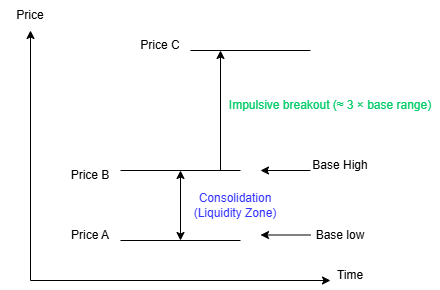
Fig. 1. Conceptual Presentation of Liquidity Demand

Our prior research approached this behavior quantitatively rather than visually. Across repeated, high-quality setups on multiple instruments and timeframes, we measured the relationship between the depth of the liquidity zone (the distance between Prices A and B) and the magnitude of the impulsive breakout (from the range boundary to Price C). A recurring proportional relationship consistently emerged from the data—most often approximating a 1:3 ratio (liquidity zone depth to breakout/impulse magnitude)—forming the statistical foundation for the model implemented and tested in this study. 

This observed ratio serves as a practical example of how institutional liquidity engineering frequently produces asymmetric expansions after consolidation phases. In many real-market instances, tighter liquidity zones (e.g., 20–40 pip ranges on lower timeframes) precede significantly larger displacement moves (often 60–120+ pips or more), where the breakout leg extends roughly three times (or greater) the prior range depth before meaningful retracement or retest. Such patterns align closely with common Smart Money Concepts (SMC) and Inner Circle Trader (ICT) observations, where liquidity sweeps enable strong impulsive continuations or reversals by harvesting clustered orders and fueling the subsequent directional phase.

That said, this proportional relationship is not a universal constant across all currency pairs, market conditions, timeframes, or volatility regimes. For example, highly trending pairs during major news events may exhibit expansions closer to 1:4 or 1:5, while choppy or ranging sessions (such as Asian consolidation on indices) often yield smaller multiples (e.g., 1:1.5–1:2.5). Asset-class differences—forex versus indices, crypto, or commodities—further introduce variability due to distinct liquidity pools, participant dynamics, and average true range characteristics.

The statistical tendency we identified, therefore, represents a high-probability guideline rather than a rigid rule. This inherent variability highlights the importance of adaptability: by incorporating an adjustable input parameter (e.g., RatioMultiplier) in the indicator, traders can empirically test and fine-tune the threshold to best suit specific symbols, timeframes, or trading styles. A setting of "3×" might perform optimally on XAUUSD M15, while "2.5×" suits GBPJPY M15, or "4×" aligns better during high-volatility periods like NFP releases.

Ultimately, the real benefit of this research lies not in pinpointing an unchanging constant, but in demonstrating that a measurable, recurring relationship exists between the size of engineered liquidity zones and the ensuing breakout impulse. Before this quantitative approach, such zones were often evaluated subjectively through visual cues like range "tightness" or wick clusters alone. By quantifying this variable, we uncover an objective edge—identifying setups where the market has historically delivered asymmetric reward potential following liquidity sweeps. This insight provides the core rationale for the indicator developed here: converting a repeatable institutional behavioral pattern into a real-time, customizable tool that enables traders to align more systematically with smart money flow.

The most consistent observation from our analysis was an approximate 1:3 ratio—the impulsive breakout leg frequently measures around three times (or more) the depth of the preceding liquidity zone. This is not presented as a rigid, universal rule, but as a high-probability guideline that aligns closely with established Smart Money Concepts (SMC) and Inner Circle Trader (ICT) market models. In practice, smaller, well-defined consolidation zones often precede larger, more explosive displacement moves once resting liquidity is swept and market structure breaks.

With this dynamic now clearly defined—liquidity zone → impulsive breakout (often ~1:3) → high-probability retest—we have a robust, repeatable framework that captures the institutional cycle of manipulation, displacement, and retracement at the heart of liquidity-driven price action.

This framework serves as the foundation for the next phase of the project: transforming theoretical insight into a practical, visual trading tool. The custom indicator we will develop is designed to:

• Automatically detect and highlight valid liquidity zones based on objective consolidation criteria.  
• Measure and track the depth of each identified zone.  
• Recognize qualifying breakouts and compute the emerging impulse range in real time.  
• Visualize the observed 1:3 relationship (with full user-adjustable ratio flexibility) directly on the chart.  
• Highlight and optionally alert potential retest zones when price returns to the original liquidity bounds after a qualifying breakout

By encoding this logic in MQL5, we shift from conceptual observation to an executable, chart-integrated model. The result is an objective tool that reduces subjectivity, filters out noise, and enables traders to better align entries with institutional order flow—ultimately enhancing timing, risk-to-reward ratios, and overall confidence in both continuation and reversal setups.

In the following section, we transition into the practical implementation, detailing the MQL5 logic, key variables, zone-detection rules, breakout validation conditions, and visualization techniques required to bring this market model to life on the chart.

Implementation

Indicator Declaration and Inputs

At the top of the indicator, we define the scope, purpose, and configurability of the tool. The indicator is designed to run directly on the chart window and exposes a focused set of inputs that control both logic and visualization. Parameters such as LookbackBars and RatioMultiplier govern how far back the algorithm searches for valid liquidity bases and how strong an impulsive move must be relative to its base. Visual inputs—including colors, opacity, buffer styles, and extension length—allow the trader to adapt the presentation without altering the underlying logic. This separation ensures the analytical model remains stable while visual preferences remain flexible.

#property indicator_chart_window
#property indicator_buffers 8
#property indicator_plots   4

input int      LookbackBars     = 500;
input double   RatioMultiplier  = 3.0;
input int      ZoneExtendBars   = 50;

input color    DemandColor      = clrLimeGreen;
input color    SupplyColor      = clrTomato;
input int      ZoneOpacity      = 40;

Global Arrays and Indicator Buffers

Next, we declare global arrays for price data and indicator buffers. Rather than relying solely on the incoming OnCalculate arrays, we explicitly copy and manage our own OHLC and time arrays. This approach gives us full control over indexing, ensures consistency when extending zones into the future, and avoids ambiguity when mapping bars to objects. The eight indicator buffers serve distinct roles: storing zone boundaries, signaling zone presence, and preserving time information for lifecycle management. This structure allows the indicator to function both visually and programmatically if later consumed by an EA or another indicator.

double OpenArr[], HighArr[], LowArr[], CloseArr[];
datetime TimeArr[];

// Buffers
double DemandHigh[], DemandLow[], SupplyHigh[], SupplyLow[];
double ZoneSignal[], ZoneStartTime[], ZoneEndTime[], ZoneType[];

Initialization Logic (OnInit)

During initialization, we normalize point values to handle both standard and fractional pricing instruments correctly. We then configure indicator metadata, bind buffers, and explicitly initialize all buffers with EMPTY_VALUE to prevent rendering artifacts. Each plot is configured independently, allowing demand and supply zones to be visually distinguished while sharing a common rendering style. Finally, any previously drawn zones are cleared to ensure the chart starts in a clean, deterministic state. This guarantees that every indicator load reflects only current calculations.

int OnInit()
{
   IndicatorSetString(INDICATOR_SHORTNAME, "Liquidity Zone 1:3 Model");

   SetIndexBuffer(0, DemandHigh, INDICATOR_DATA);
   SetIndexBuffer(1, DemandLow,  INDICATOR_DATA);
   SetIndexBuffer(2, SupplyHigh, INDICATOR_DATA);
   SetIndexBuffer(3, SupplyLow,  INDICATOR_DATA);

   SetIndexBuffer(4, ZoneSignal,    INDICATOR_CALCULATIONS);
   SetIndexBuffer(5, ZoneStartTime, INDICATOR_CALCULATIONS);
   SetIndexBuffer(6, ZoneEndTime,   INDICATOR_CALCULATIONS);
   SetIndexBuffer(7, ZoneType,      INDICATOR_CALCULATIONS);

   ArrayInitialize(DemandHigh, EMPTY_VALUE);
   ArrayInitialize(SupplyHigh, EMPTY_VALUE);

   DeleteAllZones();
   return INIT_SUCCEEDED;
}

Cleanup and Object Management (OnDeinit and DeleteAllZones)

Proper cleanup is critical for object-based indicators. When the indicator is removed or recalculated, we systematically delete all chart objects created by this tool using a strict naming convention. This prevents object accumulation, chart clutter, and performance degradation. By centralizing deletion logic in a dedicated function, we ensure consistent behavior during reinitialization, timeframe changes, or manual removal.

void OnDeinit(const int reason)
{
   DeleteAllZones();
}

void DeleteAllZones()
{
   for(int i = ObjectsTotal(0) - 1; i >= 0; i--)
   {
      string name = ObjectName(0, i);
      if(StringFind(name, "LQ_ZONE_") == 0)
         ObjectDelete(0, name);
   }
}

Utility Functions: Candle Range and Time Mapping

To keep the core logic readable and reusable, we isolate common operations into helper functions. CandleRange() abstracts the calculation of a bar’s high–low range, reinforcing clarity when comparing base and impulse candles. GetTimeForBar() ensures accurate time mapping even when extending zones beyond available historical bars. This is especially important for projecting zones into the future, where no direct bar timestamps exist yet.

double CandleRange(int index)
{
   return HighArr[index] - LowArr[index];
}

datetime GetTimeForBar(int index)
{
   if(index < ArraySize(TimeArr))
      return TimeArr[index];

   int delta = index - ArraySize(TimeArr) + 1;
   return TimeArr[ArraySize(TimeArr) - 1] + PeriodSeconds() * delta;
}

Zone Rendering Logic (DrawZone)

The DrawZone() function is responsible for translating a detected liquidity base into a visible chart object. Using the base candle’s time and price extremes, we construct a rectangle that extends forward by a user-defined number of bars. The function handles both historical and forward projection scenarios, applies appropriate coloring and opacity, and ensures objects are non-interactive and background-rendered. This keeps zones informative without interfering with manual analysis or trading actions.

void DrawZone(string name, datetime t1, datetime t2, double high, double low, color clr)
{
   ObjectCreate(0, name, OBJ_RECTANGLE, 0, t1, high, t2, low);
   ObjectSetInteger(0, name, OBJPROP_COLOR, clr);
   ObjectSetInteger(0, name, OBJPROP_BACK, true);
   ObjectSetInteger(0, name, OBJPROP_TRANSPARENCY, ZoneOpacity);
}

Buffer Population for Zones (FillZoneBuffers)

While rectangles provide visual clarity, buffers allow zones to be represented in a data-driven way. This function synchronizes buffer values with the rectangle’s lifespan, filling zone boundaries and signal markers across all bars covered by the zone. By storing start and end times in dedicated buffers, we retain full temporal awareness of each zone. This dual representation—objects for visualization and buffers for logic—makes the indicator extensible and EA-ready.

void FillZoneBuffers(int start, int end, double high, double low, bool isDemand)
{
   for(int i = start; i <= end; i++)
   {
      if(isDemand)
      {
         DemandHigh[i] = high;
         DemandLow[i]  = low;
         ZoneType[i]   = 1;
      }
      else
      {
         SupplyHigh[i] = high;
         SupplyLow[i]  = low;
         ZoneType[i]   = -1;
      }
      ZoneSignal[i] = 1;
   }
}

Buffer Maintenance (ClearOldBuffers)

Markets move forward, and zones eventually expire. This function ensures that buffer values are cleared once a zone’s projected lifetime has passed. Instead of clearing buffers blindly, we check time validity to avoid prematurely removing active zones. This approach keeps memory clean, prevents false signals, and ensures that only relevant structures remain visible and accessible.

void ClearOldBuffers(int index)
{
   if(ZoneEndTime[index] < TimeCurrent())
   {
      DemandHigh[index] = EMPTY_VALUE;
      SupplyHigh[index] = EMPTY_VALUE;
      ZoneSignal[index] = EMPTY_VALUE;
   }
}

Core Calculation Loop (OnCalculate)

The heart of the indicator resides in OnCalculate. Here, we copy the required price data, enforce series indexing, and determine how many bars should be processed based on user-defined limits. The algorithm scans historical bars looking for a simple but powerful pattern: a consolidation base followed by an impulsive candle in the same direction whose range meets or exceeds the predefined ratio threshold. When such a condition is satisfied, the base candle is classified as a valid liquidity zone and passed to the drawing and buffering routines. This logic directly implements the 1:3 liquidity-to-impulse relationship identified in our research, transforming a statistical insight into an actionable chart-based signal.

int OnCalculate(const int rates_total,
                const int prev_calculated,
                const datetime &time[],
                const double &open[],
                const double &high[],
                const double &low[],
                const double &close[])
{
   ArraySetAsSeries(time, true);
   ArraySetAsSeries(high, true);
   ArraySetAsSeries(low,  true);

   CopyTime(_Symbol, _Period, 0, LookbackBars, TimeArr);
   CopyHigh(_Symbol, _Period, 0, LookbackBars, HighArr);
   CopyLow (_Symbol, _Period, 0, LookbackBars, LowArr);

   for(int i = LookbackBars - 2; i >= 1; i--)
   {
      double baseRange   = CandleRange(i);
      double impulseRange = CandleRange(i - 1);

      if(impulseRange >= baseRange * RatioMultiplier)
      {
         bool bullish = CloseArr[i - 1] > OpenArr[i - 1];
         string name  = "LQ_ZONE_" + IntegerToString(i);

         datetime t1 = TimeArr[i];
         datetime t2 = GetTimeForBar(i + ZoneExtendBars);

         DrawZone(name, t1, t2, HighArr[i], LowArr[i],
                  bullish ? DemandColor : SupplyColor);

         FillZoneBuffers(i, i + ZoneExtendBars, HighArr[i], LowArr[i], bullish);
      }
   }
   return rates_total;
}

Final Thoughts on the Implementation

This implementation deliberately favors clarity and structural discipline over excessive optimization. Each section of logic mirrors a conceptual step in the market model: identification, validation, projection, and lifecycle management. By walking through the code in this way, the reader can clearly see how institutional behavior—consolidation, displacement, and retracement—is translated into deterministic rules. More importantly, the indicator remains adaptable: ratios can be tuned, filters can be added, and visualization can be refined without compromising the core framework.

With the logic now fully defined and implemented, the next step is to move from theory and structure into validation through testing. Having the tool on the chart allows us to observe the 1:3 base-to-impulse relationship in real market conditions, across different symbols, sessions, and volatility regimes. By deploying the indicator on multiple pairs and timeframes, we can evaluate how consistently the ratio holds, where it performs best, and where market context introduces variation. This testing phase is not about forcing the model to fit every scenario, but about gathering practical evidence, refining thresholds, and confirming that the statistical insight translates into repeatable, trade-relevant behavior once exposed to live price action.

Testing

After successful compilation with no errors, we attached the indicator to a live chart for real-time validation. In the screencast below, we demonstrate its performance on XAUUSD (Gold/USD), a highly liquid instrument where liquidity-driven structures are particularly prominent due to institutional participation.

Fig. 2. Testing the Liquidity Zone Indicator on XAUUSDmicro

The detected liquidity zones aligned remarkably well with actual price action:

• Zones were accurately placed at prior consolidation ranges.
• Breakouts from these zones consistently produced impulsive moves that respected (or exceeded) the default 1:3 ratio (zone depth to breakout magnitude), confirming the statistical foundation from our earlier research.

Most encouragingly, the default ratio setting (3.0) performed effectively out of the box on XAUUSD, with qualifying setups triggering clean, high-probability zones that matched observed institutional behavior. No immediate adjustments were required, validating that the model translates well from research to live application on this symbol.

An additional noteworthy observation is the relative rarity of qualifying setups. The strict criteria (bullish/bearish candle sequence + breakout range ≥ 3 × base range) naturally filter out marginal or noisy consolidations. This scarcity can be a deliberate advantage for traders aiming to reduce over-trading: the indicator highlights only the higher-conviction liquidity-engineered structures, encouraging patience and selective entries aligned with stronger institutional intent.

I went a step further by testing the indicator on highly volatile instruments—most notably the Volatility Index (75s). At the research-derived RatioMultiplier value of 3.0, the indicator produced very few signals. Meaningful zone detection only emerged after reducing the ratio to 2.0, although price continued to respect the identified levels through clear price-action reactions.

I observed a similar behavior on EURUSD, where only a limited number of zones were detected at the default ratio until the multiplier was adjusted downward. These observations reinforce an important conclusion: while the 1:3 ratio provides a statistically strong baseline, optimal performance requires adaptability. Different instruments respond to different impulse-to-base proportions, influenced by their inherent volatility and market structure.

This finding validates the decision to expose the ratio as a configurable input. It allows traders and researchers to vary the threshold, explore alternative ratios, and calibrate the model to specific instruments rather than forcing a single static rule. Figures 3 and 4 below illustrate these comparative results across instruments.

Fig. 3. Testing on Volatility Indices

Fig. 4. Testing on EURUSD

Conclusion

We have successfully translated the base-to-impulse ratio concept into a functional liquidity zone indicator. The results confirm a clear structural relationship between the consolidation base—whether supply or demand—and the subsequent breakout impulse. While the 1:3 ratio emerged as a strong average in our earlier research, further testing reveals that this proportion is not universal. The optimal ratio varies across instruments and market conditions, meaning that fixed settings may not perform consistently in all scenarios.

I hope this article provided practical insights. Our future work will focus on translating these concepts into a fully automated trading system, further validating the ideas through systematic testing and real-time execution. The key lessons and supporting attachments are presented below for reference.

Key Lesson

Key Lesson	Description:
The liquidity zone to breakout impulse ratio is a real, measurable pattern.	Research consistently showed a recurring relationship between the depth of consolidation/liquidity zones and the size of the subsequent impulsive breakout, most commonly around 1:3 on average across many high-quality setups.
The ratio is a high-probability guideline, not a universal constant.	While 1:3 performed well as a starting point on several instruments (e.g., XAUUSD), it varies significantly by pair, asset class, timeframe, and market conditions—requiring adjustment (e.g., 2.0 for Volatility 75 Index or choppy sessions) to capture valid, respected zones without missing opportunities or adding noise.
Flexibility through user inputs is the key to practical application.	By making the RatioMultiplier adjustable, the indicator becomes adaptable to any symbol or trading style. Traders can empirically test and optimize the value per instrument, turning a statistical observation into a personalized, objective edge that aligns with institutional liquidity behavior across diverse markets.
Higher-timeframe structure improves the reliability of liquidity zones.	Using higher timeframes to define liquidity bases and impulse magnitudes provides cleaner structures and more stable ratios. These zones tend to remain respected when price is later analyzed on lower timeframes, reinforcing the top-down nature of liquidity-driven market behavior.
Quantification transforms subjective concepts into repeatable logic.	By converting visual supply-and-demand interpretations into measurable rules—base range, impulse magnitude, and ratio thresholds—we eliminate ambiguity and enable consistent detection, backtesting, automation, and further statistical refinement.

Attachments

Source File Name

Description

Liquidity_Zone_Indicator.mq5

Custom MetaTrader 5 indicator that detects and visualizes liquidity (supply and demand) zones based on a quantified base-to-impulse relationship. The indicator identifies consolidation bases, validates breakout impulses using a configurable ratio multiplier derived from statistical research, projects zones forward on the chart, and highlights high-probability retest areas. Designed to be adaptable across instruments and timeframes, with fully adjustable parameters for testing, calibration, and further automation.

Back to contents