Uncertainty as a Model (Part 1): Random Variables — The Language of Uncertainty

Table of Contents

1. Foreword
2. Introduction
3. General Definition
4. Simple Examples
5. Distribution Function (CDF)
6. Analogy Between Probability and Mass
7. Types of Distributions
• Discrete
• Continuous
• Mixed
8. Main Characteristics
• Mean with Respect to the Distribution (Expectation)
• Quantiles
9. Conclusion
10. Appendix
• Distributions in the MQL5 Standard Library
• Comparison of Distributions Using CDF Plots
• Comparison of Distributions Using PDF Plots
• Comparing Distributions on a QQ Plot
11. Attached Files

Foreword

Probability theory and mathematical statistics are not merely “academic baggage,” but a fundamental working tool for traders. Without this framework, it is impossible to adequately model market uncertainty: any analysis — from a basic calculation of a trading strategy’s profitability to the construction of complex risk models — relies entirely on probabilistic logic.

Despite its long history, classical statistics remains at the forefront of progress. Large language models (LLMs) serve as a prime example. At their architectural core, neural networks are complex probabilistic models whose training is based on the classical maximum likelihood principle. A systematic understanding of this foundation is essential not only for analyzing market data, but also for understanding how modern AI technologies work, evaluating their effectiveness, and recognizing their fundamental limitations.

Disclaimer. It is impossible to provide an exhaustive account of the theory of random variables in a single article. We will cover only the key aspects, striking a balance between mathematical rigor and practical utility.

Introduction

There is a well-known joke in the mathematics community: “There is nothing random about random variables.” Despite the irony, this statement has profound practical significance. In a scientific context, the term “random” has almost nothing in common with its everyday meaning — as something capricious, unstable, or unfounded.

A random variable, an event, or a process is a completely deterministic mathematical object (a function or a set). They are not prone to suddenly disappearing or undergoing chaotic changes for unknown reasons. In essence, the term “random” here is nothing more than a historically established convention, which can most simply be understood as “an object studied using the methods of probability theory.” Here we have a typical example of a term that isn't particularly well-chosen, but has stuck simply because of centuries-old habit.

But this raises a valid question: if everything is so strictly defined, where, then, is chance itself hidden? It is important to understand that probability theory does not claim to be an oracle that can predict the outcome of every single experiment. It is neither magic nor foresight. Its focus is on something else:

• We do not know exactly which outcome ω will be drawn from the probability space Ω. However, we have a “map of the terrain” — we know the probabilities of events and the statistical characteristics of random variables.
• Rather than predicting a specific future, probability theory provides us with a description of the entire set of possible outcomes. We calculate parameters that do not indicate what exactly will happen right now, but rather how the system behaves in general when the experiment is repeated many times.

Thus, mathematics does not describe chaos, nor does it describe the specific outcome of a single coin toss. We work with numerical characteristics (mean, spread, distribution) that describe the entire ocean of possible outcomes, leaving the specific result of each individual experiment as an unpredictable “black box.” That is precisely why this branch of science is called “probability theory” and not “chance theory.”

General Definition

Our reasoning is based on the concept of a probability space Ω, which we discussed in the previous article. In real-world problems, we almost never know how it is “really” structured — its structure is too complex to describe directly. Therefore, in applied science, we simply postulate its existence. In practice, the information conveyed by random variables is sufficient for our purposes.

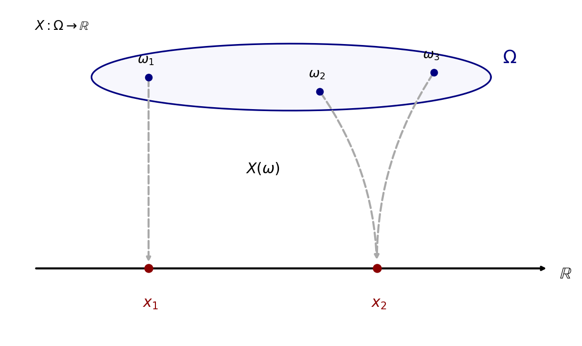
A random variable is a function X = X(ω) that assigns a well-defined number to each elementary outcome ω in the space Ω. If we are referring to a specific numerical value of this function at the point ω, a lowercase letter is used: x = X(ω). The figure below attempts to illustrate this graphically: the point ω₁ is mapped to the number x₁ (a point on the real line ℝ), while the points ω₂ and ω₃ are mapped to the same number x₂.

Distribution Function (CDF)

Every random variable X is not just a function; it is a bridge that carries probabilities from the abstract space Ω to our familiar real number line ℝ. The mechanics of this transfer are simple: the probability that the value of the random variable falls within a certain interval on the line is exactly equal to the probability of those elementary outcomes ω that “land” within that interval. To solve the vast majority of practical problems in statistics, it is quite sufficient to know how to work with such intervals and their unions.

Why is this important? Working with the “pure” space Ω is practically impossible — it is too amorphous. But as soon as we move to a distribution on the number line, we have an extremely powerful tool in our hands. Any such distribution is uniquely described by an ordinary numerical function F(x), known as the distribution function (CDF) of the random variable X. Mathematically, this is written as follows: the value of the function at the point x is the probability that the random variable will take a value not exceeding x. In other words, the distribution function (CDF) is the “cumulative” probability. It accumulates all the probabilities of events from negative infinity up to the boundary we have chosen. It is precisely this function (and its derivative — the density) that we will deal with in 99% of cases when analyzing data.

Terminological Nuances: Probability Distribution vs. the Distribution Function (CDF) of a Random Variable.

1. A probability distribution is a “rule” that assigns a probability to a set (or event). This is a more general and abstract concept.
2. A distribution function (CDF) is a specific numerical function that maps a number to another number. This is our working tool, which translates an abstract distribution into the language of graphs and formulas.

In international practice and professional literature, the distribution function is commonly called the CDF (Cumulative Distribution Function — cumulative distribution function). The word “cumulative” is key here.

Analogy Between Probability and Mass

This analogy is useful for understanding the essence: probability as mass. Imagine that the total probability, equal to one (or 100%), is a physical mass distributed (spread out or concentrated at specific points) along the real line. Following this logic, the CDF at point x shows the accumulated mass over the entire interval from -Inf to x. The farther we move to the right along the axis, the more “weight” we accumulate, until, by the time we reach positive infinity, we have collected it all (i.e., 1). This “physics of the process” is not just a metaphor. It is deeply embedded in the logic of statistical software packages and programming languages (such as R, Python, or MQL5). If you understand probability as mass, you will easily see why the probability density function is called a density (mass density), and why the expected value is called the center of mass.

Within this “mass” analogy, a degenerate random variable (which we mentioned earlier as an analogue of an ordinary number) takes on a clear physical meaning. While a typical random variable “spreads” probability along the real line, in the degenerate case the entire 100% of the mass (unit probability) is compressed into a single infinitesimally small point. Think of it as a weight sitting on a scale at a specific coordinate:

• To the left of this point, the accumulated mass is zero.
• As soon as we pass the point where the “weight” is located, the CDF value instantly jumps to one.

This perspective allows us to view ordinary numbers not as something foreign to randomness, but as a limiting, special case of a probability distribution. This understanding is extremely useful when we move on to studying the convergence of stochastic processes: chaos gradually “contracts” to a single point, turning into a predictable constant.

Simple Examples

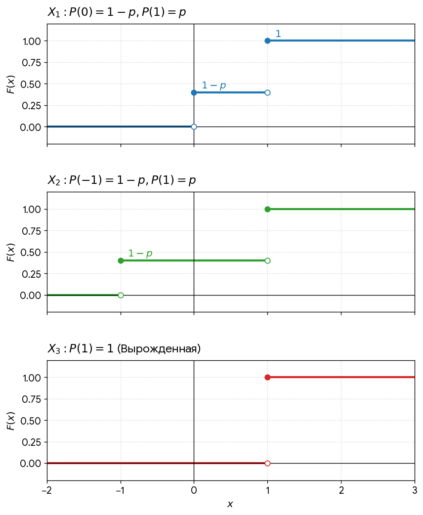
Let’s consider the simplest example — a Bernoulli scheme with n=1 (a single coin toss). We have only two elementary outcomes here, so functions on them can be defined using a table. Here are three possible variants — X1, X2 and X3:

	X1	X2	X3
ω1 = H	1	1	1
ω2 = T	0	-1	1

The third option may cause some confusion. It would seem, what is the point of a random variable that takes the same value for every outcome of a random experiment? Nevertheless, such random variables, known as degenerate random variables, are quite important in theory. Many of the most important theorems, such as the Law of Large Numbers (LLN), state that a sequence of random variables converges to a degenerate random variable. For intuitive understanding, degenerate random variables can also be viewed as analogues of ordinary (deterministic) quantities — simply familiar numbers.

Now let's construct the distribution functions (CDFs) for these three examples. The plots of these functions are shown below. All of them are discontinuous, and at the points of discontinuity their values equal the right-hand limit, which is indicated on the plots by small filled circles. Discontinuities occur at points corresponding to the values taken by the random variables. The sizes of the jumps at the discontinuities (the step heights) are equal to the probabilities of the corresponding values (in the first two plots, they are q and p, with q=1-p, and in the third plot, 1).

Types of Distributions

Discrete Distributions

The examples given above were of discrete random variables in which the probability is concentrated at a finite (or countable) number of points. In addition to the CDF, the concept of a probability mass function (PMF) is introduced for such variables. The value of this function is equal to the probability mass at a given point. In other words, it is nonzero only at a finite (or countable) number of points.

The second table in the first appendix to the article provides examples of discrete distributions with a finite number of points (binomial and hypergeometric). It also includes an example of a discrete distribution with an infinite (countable) number of points with nonzero probability: the Poisson distribution.

Calculating the probability that a random variable with a discrete distribution falls within a given interval:

1. If the PMF is known, you need to sum the probability masses for all points with nonzero probability that fall within the interval. If some points fall on an endpoint of the interval, you need to check carefully whether they are included in the interval.
2. If the CDF is known, you need to take the difference between its values at the right and left endpoints of the interval. Here, too, you need to account for whether points with nonzero probability are included, depending on the type of interval. It is also important to know exactly how the CDF is defined in the particular statistical package being used — there are cases where a strict inequality is used in its definition.

Continuous Distributions

A distribution function (CDF) need not have discontinuities and may well be continuous. The simplest example is a uniform distribution on the interval from zero to one. The probability that the random point falls in any interval equals the length of its intersection with the interval [0, 1]. The distribution of the random variable X (the coordinate of a random point) is specified by the CDF F(x), such that F(x) = 0 for x < 0, F(x) = x for 0 ≤ x < 1, and F(x) = 1 for x ≥ 1. The graph of this function is shown below.

For continuous random variables, another essential tool is introduced: the probability density function (PDF). Mathematically, the density is the derivative of the distribution function F(x). To continue our physical analogy, if F(x) is the total mass over an interval, then the PDF is the intensity with which this mass is “spread out” along the real line. Let's take our example (a uniform distribution on the interval [0, 1]): outside this interval, the density is zero (it is “empty” there; there is no mass). Inside the interval, the density is equal to one (the mass is distributed in a perfectly uniform layer). The graph of this function is shown below.

This often raises a valid question: what about points of discontinuity? In our example, the density jumps instantly from 0 to 1 at the endpoints of the interval. Which PDF value should we choose there — 0, 1 or 0.5? The mathematical answer eliminates the need to choose: for continuous distributions, it makes no difference. Unlike discrete random variables, where probability mass can be “concentrated” at a single point, in the continuous world the probability at any given point is always zero. Probability makes sense here only for intervals. Think of it as trying to measure the weight of a geometric point on a line: no matter how many points you take, their total weight will only become apparent when they make up an interval. Therefore, we can assign any value at the points of discontinuity — this will have no effect on the final probability calculation (the integral).

To better understand the concept of density, it is helpful to use an intuitive technique that transforms a complex continuous distribution into an understandable discrete model. This method is the foundation of any computer simulation (such as the Monte Carlo method). Imagine that we “slice” the continuous number line into tiny intervals of length d. Now we can make an assumption: at each such point x, the probability concentrated there is not zero, but some small approximate probability P. This probability is calculated as the product of the density and the step width: P~p(x)*d. Why does this work? If the density p(x) is the “height” of the graph at a given point, and d is its “width,” then their product is the area of a thin rectangle. The sum of all such rectangles (the Riemann sum) will, in the limit, give us that same probability of one (the total mass). What is the practical benefit of this model?

• For programmers: this is exactly how numerical integration algorithms work. We replace a continuous construction with a finite number of very small steps.
• For traders: market quotes are discrete in nature (the minimum price increment is a tick).

When considering the probability density through the lens of small increments d, we move from pure mathematics to the reality of a trading terminal. This perspective allows us to interpret the density p(x) not merely as an abstract derivative, but as a coefficient that increases the probability associated with a specific neighborhood of the point x. The higher the density, the greater the “chances” of ending up in that neighborhood.

The appendix to this article contains MQL5 scripts that generate plots of the CDF and PDF. For clarity, plots are provided for different distributions (normal and Cauchy).

Calculating the probability that a random variable with a continuous distribution falls within a given interval:

1. If the PDF is known, then we need to evaluate the integral of this function over the interval. We do not pay attention to the density values at individual points.
2. If the CDF is known, you need to take the difference between its values at the right and left endpoints of the interval. There are no discontinuities here (no steps). The appendix to this article contains an MQL5 script for calculating probability in such a case (a normal distribution is used as an example).

Mixed Distributions

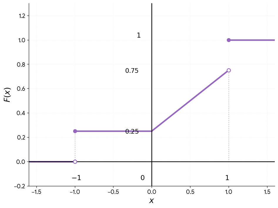
In textbooks, random variables are often divided into two strict categories: discrete variables with sharp jumps and continuous variables with smooth lines. However, reality — and trading is a good example here — is not always so clear-cut. There are mixed distributions that behave like hybrids. Mathematically, this looks like creating a “cocktail” from two different cumulative distribution functions (CDFs), F1(x) and F2(x). We can mix them in any proportions k1 and k2 (as long as they are positive and their sum equals 1): F(x)=k1*F1(x)+k2*F2(x).

The reverse is also true: virtually any “meaningful” distribution function, that is, a CDF applicable in practice, can be decomposed into continuous and discrete components. This is not just a mathematical trick. Mixed distributions are standard, for example, in reliability theory and survival analysis. A real-life example: imagine an insured event or the execution of a trading order. There is a continuous distribution of possible profit or loss, but there is also a nonzero (discrete) probability that the event will not occur at all (the loss is exactly zero) or that a fixed loss limit will be triggered.

The plot below shows such a “mixture” in a 50/50 (k1=k2=0.5) proportion. We took a smooth uniform distribution and added discrete “spikes” from our coin example to it (we used the case where the values -1 and 1 occur with equal probability p=0.5). Where the graph is sloped, the continuous component is active. Where a vertical jump is visible, the discrete probability mass at a specific value “pops up.” Understanding such hybrids is critical when working with market data, where “smooth” price movements are constantly interrupted by discrete events — gaps, clearing events, or the execution of large orders at a single price.

Calculating the probability that a random variable with a mixed distribution falls within a given interval: for each component of the mixture, we calculate the probability separately using an appropriate method. Then we sum these intermediate probabilities, with the corresponding weights, to obtain the resulting probability.

Main Characteristics of One-Dimensional Distributions

Mean with Respect to the Distribution

Rather than describing a random variable using an infinite set of points or a complex function graph, mathematicians use concise “summaries” — numerical characteristics. The most important of these is the mean of a function f(x) with respect to the distribution.

A Stieltjes integral can be defined for any CDF. Behind this intimidating name lies a powerful mathematical framework (Riemann–Stieltjes or Lebesgue–Stieltjes integrals) that allows one to work uniformly with any type of quantity. The integral of a certain numerical function f(x) with respect to a given distribution P (if it exists) is called the mean of that function.

Despite the complexity “under the hood,” for applied problems it is enough for us to understand what this integral actually amounts to in practice:

• Discrete case: the integral becomes a simple sum. We simply multiply the value of the function at each point by the probability mass at that point and add the results together.
• Continuous case: the Stieltjes integral becomes a classical definite integral of the product of our function and the probability density p(x).
• Mixed case: the principle of linearity applies here. The mean is calculated as a weighted sum of the means for each component (continuous and discrete), taking their weights into account.

Let's consider a few examples of the physical and statistical meanings that mean values take on depending on the type of function f(x) for which the mean is being calculated:

• The mean of the unit constant: f(x)=1. It is always equal to one. This is a fundamental property of “normalization”: the total probability mass (the area under the curve) must equal 100%. If that is not the case, then we are not dealing with probability.
• Expected value: f(x)=x. This is the “center of mass” of the distribution. However, it is important to remember that there are some tricky exceptions in probability theory. There are distributions (such as the Cauchy distribution) whose tails are so heavy that the integral diverges. In such cases, the expected value is simply undefined — the system has no single “center” around which it stabilizes.
• Variance: f(x)=(x-m)^2. where m is the expected value. Variance is a measure of how “spread out” the data are. It shows how much the values deviate from the center. For a degenerate random variable (a constant), the variance is zero (there is no spread). In trading, variance is the foundation for understanding volatility and risk.
• Central moments: f(x) = (x - m)^n. When n>2, we obtain higher-order numerical characteristics. For example, the third moment reflects asymmetry (the skew of the graph), while the fourth moment reflects kurtosis (the sharpness of the peak and the “heaviness” of the tails). The appendix to this article includes an example of an MQL5 script for calculating the expected value, variance, and third- and fourth-order central moments.
• Characteristic function: f(x) = exp(i*t*x), where i is the imaginary unit. Here we enter the realm of complex numbers. For continuous variables, this is nothing more than the Fourier transform of the probability density. Although the characteristic function is rarely encountered in applied statistics, it is the “holy grail” of probability theory. It is characteristic functions that are used to prove the Central Limit Theorem (CLT) — the foundation that explains why there are so many normal distributions in the world.
• To calculate the expected value of a derived quantity Y = g(X), one formally must first find its own probability density function (PDF). In practice, however, a simpler approach is used: compute the mean of g(x) with respect to the original distribution of X. The validity of this approach is not self-evident; it follows from a mathematical theorem with a rather complex proof. In Western literature, this statement has been given the ironic nickname “The Law of the Lazy Statistician” (LOTUS).

Quantiles

While the expected value indicates the “center of mass,” quantiles help us understand exactly how the mass is distributed along the number line.

In the case of a continuous distribution with CDF)F(x), the q-quantile is determined quite simply: we solve the equation F(x) = q, where q is a given probability level (from 0 to 1). The resulting value x=x(q) will be the q-quantile. In statistical packages, this function is often called the PPF (Percent Point Function) or the inverse distribution function.

Intuitively, the q-quantile is a point on the number line that “cuts off” a proportion q of the total probability mass to its left.

Here is an example for clarity: suppose we are analyzing the daily volatility of an asset in points. If the 0.9-quantile is 150 points, this means:

• On 90% of trading days, volatility will not exceed 150 points.
• In the remaining 10% of cases, the market will move by more than 150 points.

With discrete distributions (where the CDF)F(x) consists of “steps”), things are a bit more complicated. In this case, the equation F(x)=q may either have no solutions at all (if q falls on a “vertical jump”) or have infinitely many solutions (on flat sections). Nevertheless, quantiles are still defined here as well, using special rounding or interpolation rules.

Some values of q are so important that they have their own names:

• For q=0.5 — the median. The point that divides the distribution in half. Unlike the mean, the median is resistant to “outliers” and anomalous tails and is therefore often used as its robust counterpart.
• For q=0.25 and q=0.75 — the quartiles. They cut off quarters of the distribution (the lower and upper quartiles). The difference between them is called the interquartile range and, by analogy with the median, is often used as a robust counterpart to variance.
• Multiples of 0.1 — deciles.
• Multiples of 0.01 — percentiles. Market risks are most often measured in percentiles (for example, the notorious Value-at-Risk, or VaR).

The appendix to the article provides an MQL5 script for calculating a quantile for a normal distribution.

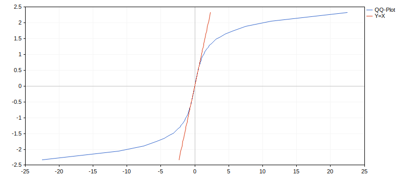
A quantile-based QQ plot (quantile-quantile plot) is often used to visually compare two distributions. This is a two-dimensional plot in which each point corresponds to the q-quantiles of the distributions. If the distributions coincide perfectly, this graph coincides with the line y = x. A QQ plot helps visually distinguish between distributions much better than their overlaid PDF or CDF plots. The appendix to this article includes an MQL5 script that plots such a graph for the Cauchy and Gaussian distributions.

Conclusion

Random variables are the fundamental language used to describe uncertainty in real-world systems. For a trader, analyst, or developer of trading algorithms, this framework is not an abstract theory, but a practical tool. Through CDFs, PDFs, moments, and quantiles, we can move from chaotic market observations to numerical characteristics: risk assessment, the probability of extreme movements, the robustness of strategies, and the statistical properties of the data.

The practical value of this approach lies in the fact that most market analysis tasks boil down to working with distributions. Understanding how CDFs, PDFs, and quantiles work allows you to correctly calculate probabilities, construct risk metrics, compare models, and analyze data structure. Using the built-in statistical functions of the MQL5 Standard Library makes these tools available directly within trading applications and research scripts.

However, in real-world problems, a single random variable is almost never enough. We are interested in the relationships between them: the joint behavior of prices, returns, volatility, and other factors. Therefore, the next step will be to study multidimensional random variables, where joint distributions and the structure of dependencies between variables play a key role.

Appendices: Practical Implementation in Code

This section contains code examples that illustrate the key concepts of the article. We deliberately set them apart from the main narrative so that the technical details of the implementation would not distract from the mathematical logic of the discussion.

Appendix 1

A table listing some continuous distributions and links to the related functions in the Statistics section of the MQL5 Standard Library. It is convenient that there are vectorized counterparts for distribution functions, probability density functions (PDFs), and quantile functions. To use each distribution, you need to include the corresponding header files. For example, for the normal distribution:

//--- Include the normal distribution functions
#include <Math\Stat\Normal.mqh>

Name of the distribution family	Distribution function (CDF)	Probability density function (PDF) / density	Inverse distribution function (quantile function, Percent Point Function, PPF)	Comment
Gaussian (normal)	MathCumulativeDistributionNormal()	MathProbabilityDensityNormal()	MathQuantileNormal()	It is often used as a benchmark for comparison with distributions of price increments (or log returns)
Lognormal	MathCumulativeDistributionLognormal()	MathProbabilityDensityLognormal()	MathQuantileLognormal()	The distribution of a quantity whose logarithm follows a normal distribution. It is often used as a benchmark for comparison with distributions of price returns
t-distribution (Student’s t-distribution)	MathCumulativeDistributionT()	MathProbabilityDensityT()	MathQuantileT()	The best-known application is interval estimation of the expected value for a normally distributed sample.
Chi-square distribution (Pearson distribution)	MathCumulativeDistributionChiSquare()	MathProbabilityDensityChiSquare()	MathQuantileChiSquare()	Its best-known application is the goodness-of-fit test of the same name.
F-distribution (Fisher distribution)	MathCumulativeDistributionF()	MathProbabilityDensityF()	MathQuantileF()	Used in the F-test
Cauchy distribution	MathCumulativeDistributionCauchy()	MathProbabilityDensityCauchy()	MathQuantileCauchy()	It is known for lacking, in the usual sense, an expected value and moments

The same applies to several discrete distributions:

Name of the distribution family	Distribution function (CDF)	Probability mass function (PMF)	Comment
Binomial distribution	MathCumulativeDistributionBinomial()	MathProbabilityDensityBinomial()	Used to test hypotheses about the probability of an event
Hypergeometric distribution	MathCumulativeDistributionHypergeometric()	MathProbabilityDensityHypergeometric()	Used in Fisher’s exact test
Poisson distribution	MathCumulativeDistributionPoisson()	MathProbabilityDensityPoisson()	It can model, for example, the distribution of the number of price ticks per unit time (parameter: mean intensity)

Appendix 2

The p_calc.mq5 script calculates the probability that a normally distributed random variable falls within a specified interval. The distribution parameters and interval boundaries are specified as input data. Calculation result:

For a normal distribution with a mean of 0.50 and a standard deviation of 1.60, the probability of falling within the interval from 0.20 to 1.70 is 0.35.

Appendix 3

The moments.mq5 script for calculating the first four moments of the exponential distribution. It should be noted that, from a formal standpoint, the coefficients of skewness and kurtosis are not the central moments themselves, but their dimensionless counterparts (normalized by the standard deviation). The mean of the exponential distribution is specified as an input parameter. Calculation result:

For the exponential distribution with a mean of 0.50:
Expected value 0.50
Variance 0.25
Skewness 2.00
Kurtosis 6.00

Appendix 4

The q_calc.mq5 script for calculating the quantile of a normally distributed random variable. The distribution parameters and the probability for which the quantile is to be calculated are specified as input data. Calculation result:

For a normal distribution with a mean of 0.50 and a standard deviation of 1.60, the quantile corresponding to a probability of 0.20 is -0.85.

Appendix 5

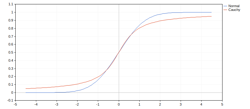
The two_cdf.mq5 script plots the cumulative distribution functions (CDFs) for the Gaussian and Cauchy distributions on a single set of coordinate axes. For the normal distribution, the standard parameters (0, 1) were chosen, and for the Cauchy distribution, (0, 0.7) were chosen, so that they would correspond better to each other (their centers coincide and their interquartile ranges are nearly equal). The difference between the plots is noticeable, but what it represents is not obvious. For example, we might mistakenly assume that two distributions with different parameters were simply chosen from the same family.

Appendix 6

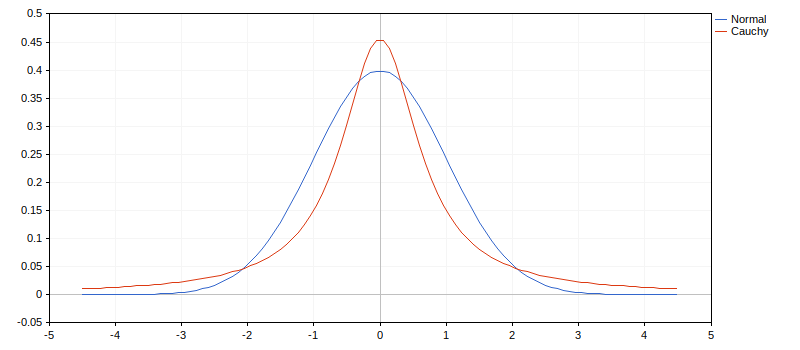
The two_pdf.mq5 script plots the probability density functions for the same two distributions (as in the previous appendix). The difference is slightly more obvious, but it is still difficult to interpret (especially in the tails).

Appendix 7

The qqplot_theoretical.mq5 script plots a QQ plot for the same two distributions (as in the two previous appendices). For comparison, here is a graph of the line y = x. There is now no doubt whatsoever that these are completely different distributions, with significantly different behavior in the tails. The assumption that these are two normal distributions with different parameters can be rejected — in that case, the graph would be a segment of the straight line y = ax + b (which is clearly not observed).

Attached Files

#	name	Description
1	p_calc.mq5	Script for calculating the probability that a random variable with a normal distribution falls within a specified interval
2	moments.mq5	Script for calculating the first four moments of the exponential distribution
3	q_calc.mq5	Script for calculating the quantile of a random variable with a normal distribution
4	two_cdf.mq5	Script that plots the cumulative distribution functions (CDFs) for the Cauchy and Gaussian distributions on a single set of axes.
5	two_pdf.mq5	Script that plots the probability density functions (PDFs) for the Cauchy and Gaussian distributions on a single set of axes.
6	qqplot_theoretical.mq5	Script that plots a QQ plot for the Cauchy and Gaussian distributions.