Testing for Residual Autocorrelation with the Ljung-Box Portmanteau Test in MQL5

Introduction

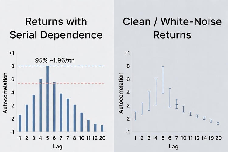
You've built a strategy. The equity curve looks nice, the return distribution seems reasonable, and when you eyeball a plot of returns over time nothing obviously screams "pattern." But "doesn't obviously scream pattern" doesn't mean there's no serial autocorrelation hiding in the data. A small lag-1 correlation tells you nothing about dependence at lag 2, 5, or 10. If you fit a model to returns (ARIMA, GARCH, or another time-series model), the residuals should show no significant autocorrelation. If they do, your model may still be missing some of the serial structure it was supposed to capture.

The tool for this job is the Ljung-Box portmanteau test. Instead of checking one autocorrelation at a time, it checks a whole block of lags together and gives you a single p-value: is there evidence of autocorrelation somewhere in this range of lags, or not?

This article presents an MQL5 implementation (LjungBoxToolkit.mq5) with no external dependencies. It computes sample autocorrelations, the Ljung-Box Q statistic, degrees of freedom, and a chi-square-approximation p-value, then prints a plain-language report to the Experts tab. It works on raw price returns, on your closed-trade history, or on an external residual series you export from any model you've already fitted.

Terminology note: In this article, autocorrelation refers specifically to the correlation between a series and its lagged values. I use serial dependence more broadly to describe dependence between observations across time. Since the Ljung-Box test is built from sample autocorrelations, autocorrelation is the primary term used throughout the article.

Why This Matters

There are three practical reasons I would run this test instead of relying on a visual scan:

1. Missed structure. If your "random-looking" returns actually carry significant autocorrelation at some lag, there may be a forecastable component or some other pattern worth investigating. That doesn't automatically make it a trading edge, but it tells you the data may not be as random as it first looked.
   
2. Model misspecification. If you've fit a model and the residuals still show significant autocorrelation, the model may still be leaving some serial structure behind. That's a warning sign that the model hasn't captured everything it was meant to capture.
   
3. Downstream statistics can be affected. Some performance and statistical tests assume independent observations, while others need to be adjusted when returns are autocorrelated. If you ignore autocorrelation, those results can be more misleading than they look.
   

One Correlation vs. a Portmanteau Test

Looking at a single autocorrelation, say ρ(1), and asking "is this significantly different from zero?" only tests one lag. Autocorrelation in financial data is often spread thinly across several lags — a bit of momentum at lag 1, a bit of mean reversion at lag 5, or some calendar-related pattern showing up at a particular horizon. On daily data, for example, lag 5 roughly lines up with one trading week. None of the individual correlations might look large enough to flag on their own, yet together they can be jointly significant.

A portmanteau test combines several autocorrelations into one statistic. The Ljung-Box version is the most widely used because it has better small-sample behavior than its predecessor, the Box-Pierce test.

The Ljung-Box Q Statistic

For a series of length n with sample autocorrelations ρ(k), the Ljung-Box statistic for lags 1 through h is:

Q(h) = n (n + 2) * Σ [ρ(k)² / (n − k)],  for k = 1 to h

Under the null hypothesis H₀ that there is no autocorrelation up to lag h, Q(h) is asymptotically compared with a chi-square distribution. For a raw, unadjusted series, the usual degrees of freedom are h. When you're testing residuals from a fitted model, the degrees of freedom may need to be adjusted because the model has already estimated some of the structure in the data. For a standard ARMA(p,q) residual test, a common adjustment is h − p − q. The exact adjustment depends on the model, so simply subtracting every fitted parameter is not always the right rule.

A large Q relative to its chi-square distribution means the observed autocorrelations are collectively too large to be explained by sampling noise alone, so we reject H0. A small Q means the observed autocorrelations are not large enough for this test to reject H0 — fail to reject the null. MQL5 does not provide a built-in chi-square CDF, so the script calculates the p-value using the regularized incomplete gamma function.

Toolkit Architecture

The script is organized into six main stages:

OnStart()
 ├─ Build the series (price returns | deal history | external file)
 ├─ ComputeAutocorrelations()   → rho[1..MaxLag]
 ├─ ParseLagSet()               → which horizons to actually test
 ├─ LjungBoxQ()  (per horizon)  → Q statistic
 ├─ ChiSquarePValue()           → p-value via GammQ/GSER/GCF/GammLn
 └─ PrintReport()               → formatted Experts-tab output

The script has three interchangeable data sources so the exact same statistical engine can be pointed at raw returns or at the leftover residuals of any model you've already built.

Step-by-Step Code Walkthrough

1. Inputs and the data-source switch

//--- data source options
enum ENUM_DATA_SOURCE
  {
   DATA_PRICE_RETURNS = 0,   // Returns from price history (Close-to-Close)
   DATA_DEAL_HISTORY  = 1,   // Returns from closed deal history (realized P/L)
   DATA_EXTERNAL_FILE = 2    // External residual series (CSV/TXT in MQL5\Files)
  };

//--- inputs
input string            InpSymbol            = "";                 // Symbol ("" = current chart symbol)
input ENUM_TIMEFRAMES   InpTimeframe         = PERIOD_CURRENT;     // Timeframe (price-return source only)
input int               InpBars              = 500;                // Bars/Deals to evaluate (ignored for external-file source)
input ENUM_DATA_SOURCE  InpDataSource        = DATA_PRICE_RETURNS; // Data source
input bool              InpUseLogReturns     = true;               // Use log returns (price source only)
input string            InpExternalFileName  = "residuals.csv";    // External residual file (in MQL5\Files)
input int               InpMaxLag            = 20;                 // Maximum lag for ACF computation
input string            InpLagSet            = "5,10,15,20";       // Lag horizons to test (comma-separated)
input int               InpDfAdjustment      = 0;                  // df adjustment; set consistently with the fitted model used for residual diagnostics
input double            InpSignificanceLevel = 0.05;               // Significance level (alpha)

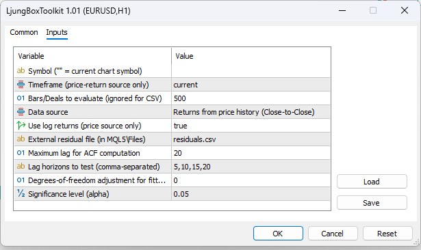
Every input maps directly onto a decision you'd have to make when running the test by hand:

• InpDataSource decides what series gets tested, which is what lets the same tool work with both raw returns and residuals from a fitted model.

• InpBars sets the number of price bars or most recent matching closing deals used to build the selected series. It applies to the price-return and deal-history sources, while the external-file source uses all values loaded from the file.

• InpMaxLag sets how far out the autocorrelation function (ACF) gets computed.

• InpLagSet lets you test several horizons in one run (e.g., "does dependence show up by lag 5? By lag 20?") without re-running the script.

• InpDfAdjustment controls the degrees-of-freedom adjustment when testing residuals from a fitted model. It must be chosen consistently with the model that produced the residuals. For a standard ARMA(p,q) residual diagnostic, the conventional adjustment is p + q, giving df = h − p − q. This is not a universal rule for every model: other models may require a different adjustment, so the appropriate value should be determined from the model and diagnostic procedure being used. Leave InpDfAdjustment at 0 for raw returns or other unadjusted series.

2. The gamma-function machinery

There's no built-in chi-square CDF in MQL5, so the p-value has to be computed by hand. The classic route, borrowed from Numerical Recipes, is the regularized incomplete gamma function — since a chi-square distribution is just a special case of the gamma distribution.

//+------------------------------------------------------------------+
//| Log-gamma function (Lanczos approximation)                       |
//+------------------------------------------------------------------+
double GammLn(double xx)
  {
   double cof[6] =
     {
      76.18009172947146, -86.50532032941677, 24.01409824083091,
      -1.231739572450155, 0.1208650973866179e-2, -0.5395239384953e-5
     };
   double x = xx;
   double y = xx;
   double tmp = x + 5.5;
   tmp -= (x + 0.5) * MathLog(tmp);
   double ser = 1.000000000190015;
   for(int j = 0; j < 6; j++)
     {
      y += 1.0;
      ser += cof[j] / y;
     }
   return -tmp + MathLog(2.5066282746310005 * ser / x);
  }

//+------------------------------------------------------------------+
//| Series expansion for the lower incomplete gamma function P(a,x)  |
//+------------------------------------------------------------------+
void GSER(double &gamser, double a, double x, double &gln)
  {
   gln = GammLn(a);
   if(x <= 0.0)
     {
      gamser = 0.0;
      return;
     }
   double ap  = a;
   double sum = 1.0 / a;
   double del = sum;
   int n;
   for(n = 1; n <= GB_ITMAX; n++)
     {
      ap += 1.0;
      del *= x / ap;
      sum += del;
      if(MathAbs(del) < MathAbs(sum) * GB_EPS)
         break;
     }
   if(n > GB_ITMAX)
      Print("LjungBoxToolkit Warning: GSER did not converge after ", GB_ITMAX,
            " iterations (a=", a, ", x=", x, "). P-value may be inaccurate.");
   gamser = sum * MathExp(-x + a * MathLog(x) - gln);
  }

//+------------------------------------------------------------------+
//| Continued fraction for the upper incomplete gamma function Q(a,x)|
//+------------------------------------------------------------------+
void GCF(double &gammcf, double a, double x, double &gln)
  {
   gln = GammLn(a);
   double b = x + 1.0 - a;
   double c = 1.0 / GB_FPMIN;
   double d = 1.0 / b;
   double h = d;
   int i;
   for(i = 1; i <= GB_ITMAX; i++)
     {
      double an = -i * (i - a);
      b += 2.0;
      d = an * d + b;
      if(MathAbs(d) < GB_FPMIN)
         d = GB_FPMIN;
      c = b + an / c;
      if(MathAbs(c) < GB_FPMIN)
         c = GB_FPMIN;
      d = 1.0 / d;
      double del = d * c;
      h *= del;
      if(MathAbs(del - 1.0) < GB_EPS)
         break;
     }
   if(i > GB_ITMAX)
      Print("LjungBoxToolkit Warning: GCF did not converge after ", GB_ITMAX,
            " iterations (a=", a, ", x=", x, "). P-value may be inaccurate.");
   gammcf = MathExp(-x + a * MathLog(x) - gln) * h;
  }

//+------------------------------------------------------------------+
//| Regularized upper incomplete gamma function Q(a,x)               |
//+------------------------------------------------------------------+
double GammQ(double a, double x)
  {
   double gamser, gammcf, gln;
   if(x < 0.0 || a <= 0.0)
      return 1.0;
   if(x < a + 1.0)
     {
      GSER(gamser, a, x, gln);
      return 1.0 - gamser;
     }
   else
     {
      GCF(gammcf, a, x, gln);
      return gammcf;
     }
  }

GammLn computes the natural log of the gamma function using a Lanczos approximation — needed because the gamma function itself overflows quickly for the values we will use.

GSER and GCF calculate the incomplete gamma function using two different numerical methods. GSER uses a series expansion when x < a + 1, while GCF uses a continued fraction when x >= a + 1. Choosing between them this way improves numerical stability. GammQ selects the appropriate method and returns the upper regularized incomplete gamma function, Q(a, x) — exactly what we need to calculate the right-tail probability for the chi-square statistic.
The routines also have an iteration limit; if either numerical method fails to converge after GB_ITMAX iterations, it prints a warning rather than silently returning a questionable p-value.

//+------------------------------------------------------------------+
//| Right-tail p-value of a Chi-square distribution                  |
//+------------------------------------------------------------------+
double ChiSquarePValue(double chiStat, double df)
  {
   if(df <= 0.0)
      return 1.0;
   double a = df / 2.0;
   double x = chiStat / 2.0;
   if(x <= 0.0)
      return 1.0;
   return GammQ(a, x);
  }

This is the payoff function: a chi-square distribution with df degrees of freedom is a gamma distribution with shape df/2 and scale 2, so P(χ² > chiStat) = Q(df/2, chiStat/2). That's our p-value.

3. Building the series — three sources

Price returns:

//+------------------------------------------------------------------+
//| Build a return series from price history                         |
//+------------------------------------------------------------------+
bool BuildReturnsFromPrice(double &out[])
  {
   string sym  = (InpSymbol == "") ? _Symbol : InpSymbol;
   int    need = InpBars + 1;

   MqlRates rates[];
   ArraySetAsSeries(rates, false);
   int copied = CopyRates(sym, InpTimeframe, 1, need, rates);
   if(copied < 11)
     {
      Print("LjungBoxToolkit: could not copy enough price data for ", sym,
            " (got ", copied, " bars). Error: ", GetLastError());
      return false;
     }

   int m = copied - 1;
   ArrayResize(out, m);
   for(int i = 1; i < copied; i++)
     {
      double p0 = rates[i - 1].close;
      double p1 = rates[i].close;
      if(p0 <= 0.0)
        {
         out[i - 1] = 0.0;
         continue;
        }
      out[i - 1] = InpUseLogReturns ? MathLog(p1 / p0) : (p1 - p0) / p0;
     }
   return true;
  }

Note ArraySetAsSeries(rates, false) keeps the copied rates in chronological order (oldest first). The data is requested starting from shift 1, so the current forming bar (Bar 0) is excluded and only closed bars are used. This makes the return series reproducible: the observations do not change depending on when the script is executed within the current bar. Each return is then calculated from one closed-bar price to the next.

Deal history:

//+------------------------------------------------------------------+
//| Build a realized P/L series from closed deal history             |
//+------------------------------------------------------------------+
bool BuildReturnsFromDeals(double &out[])
  {
   if(!HistorySelect(0, TimeCurrent()))
     {
      Print("LjungBoxToolkit: HistorySelect failed. Error: ", GetLastError());
      return false;
     }

   int total = HistoryDealsTotal();
   datetime tmp_time[];
   double   tmp_profit[];
   ArrayResize(tmp_time, 0);
   ArrayResize(tmp_profit, 0);

   for(int i = 0; i < total; i++)
     {
      ulong ticket = HistoryDealGetTicket(i);
      if(ticket == 0)
         continue;

      long entry = HistoryDealGetInteger(ticket, DEAL_ENTRY);
      if(entry != DEAL_ENTRY_OUT)
         continue; // only closing deals carry a realized result

      if(InpSymbol != "")
        {
         string dsym = HistoryDealGetString(ticket, DEAL_SYMBOL);
         if(dsym != InpSymbol)
            continue;
        }

      double profit = HistoryDealGetDouble(ticket, DEAL_PROFIT)
                      + HistoryDealGetDouble(ticket, DEAL_SWAP)
                      + HistoryDealGetDouble(ticket, DEAL_COMMISSION);
      datetime dtime = (datetime)HistoryDealGetInteger(ticket, DEAL_TIME);

      int sz = ArraySize(tmp_profit);
      ArrayResize(tmp_time, sz + 1);
      ArrayResize(tmp_profit, sz + 1);
      tmp_time[sz]   = dtime;
      tmp_profit[sz] = profit;
     }

   int cnt = ArraySize(tmp_profit);
   if(cnt < 11)
     {
      Print("LjungBoxToolkit: not enough closed deals found (", cnt, ").");
      return false;
     }

//--- sort chronologically (ascending by deal time) using an index array,
//--- since ArraySort only works on flat primitive arrays, not parallel pairs
   int idx[];
   ArrayResize(idx, cnt);
   for(int i = 0; i < cnt; i++)
      idx[i] = i;

   for(int i = 0; i < cnt - 1; i++)
     {
      int min_j = i;
      for(int j = i + 1; j < cnt; j++)
        {
         if(tmp_time[idx[j]] < tmp_time[idx[min_j]])
            min_j = j;
        }
      if(min_j != i)
        {
         int t = idx[i];
         idx[i] = idx[min_j];
         idx[min_j] = t;
        }
     }

   double sorted[];
   ArrayResize(sorted, cnt);
   for(int i = 0; i < cnt; i++)
      sorted[i] = tmp_profit[idx[i]];

   int use   = MathMin(cnt, InpBars);
   int start = cnt - use;
   ArrayResize(out, use);
   for(int i = 0; i < use; i++)
      out[i] = sorted[start + i];

   return true;
  }

This walks the account's deal history, keeps only closing deals (DEAL_ENTRY_OUT), optionally filters by symbol, and treats each selected closing deal's net realized P/L as one observation in the series. If a position is closed in multiple partial deals, each closing deal is treated separately rather than being combined into one position-level result. This is a different kind of series from fixed-interval price returns: each observation is the realized monetary P/L from a closing deal. The Deal History mode should therefore be interpreted as a test of serial dependence in realized monetary P/L, not as a test of autocorrelation in normalized strategy returns.

Because the observations are measured in absolute monetary terms, changes in position size can affect the result. If position sizing varies systematically over time, the Ljung-Box test may detect dependence partly associated with the sizing process rather than with the underlying trade outcomes themselves. For example, a strategy that increases its lot size after a sequence of trades can introduce serial structure into the monetary P/L series even if the underlying per-unit trade outcomes are not serially dependent. If the goal is specifically to study dependence in strategy returns, a suitably normalized return or per-unit outcome series should be tested instead.

This can still be useful for asking whether realized P/L observations tend to cluster or show a pattern, but it should not be interpreted as the same thing as autocorrelation in equally spaced market returns.

External file (the model-residuals path):

//+------------------------------------------------------------------+
//| Validate that a token is a well-formed numeric literal           |
//| Accepts: optional sign, digits, at most one decimal point,       |
//| optional exponent (e/E) with optional sign and required digits   |
//+------------------------------------------------------------------+
bool IsNumericToken(const string s)
  {
   int len = StringLen(s);
   if(len == 0)
      return false;

   int  i           = 0;
   bool has_digit    = false;
   bool has_dot      = false;
   bool has_exponent = false;

//--- optional leading sign
   ushort ch = StringGetCharacter(s, i);
   if(ch == '-' || ch == '+')
      i++;

//--- mantissa: digits and at most one decimal point
   for(; i < len; i++)
     {
      ch = StringGetCharacter(s, i);

      if(ch >= '0' && ch <= '9')
        {
         has_digit = true;
         continue;
        }

      if(ch == '.')
        {
         if(has_dot || has_exponent)
            return false;   // second dot, or dot after exponent started
         has_dot = true;
         continue;
        }

      if(ch == 'e' || ch == 'E')
        {
         if(has_exponent || !has_digit)
            return false;   // second exponent, or exponent with no mantissa digits yet
         has_exponent = true;

         //--- optional sign right after the exponent marker
         if(i + 1 < len)
           {
            ushort next = StringGetCharacter(s, i + 1);
            if(next == '-' || next == '+')
               i++;
           }

         //--- exponent must be followed by at least one digit
         if(i + 1 >= len || StringGetCharacter(s, i + 1) < '0' || StringGetCharacter(s, i + 1) > '9')
            return false;
         continue;
        }

      return false; // any other character disqualifies this token
     }

   return has_digit;
  }

//+------------------------------------------------------------------+
//| Load an external residual series from MQL5\Files                 |
//+------------------------------------------------------------------+
bool LoadExternalResiduals(double &out[])
  {
   int handle = FileOpen(InpExternalFileName, FILE_READ | FILE_TXT | FILE_ANSI);
   if(handle == INVALID_HANDLE)
     {
      Print("LjungBoxToolkit: cannot open file '", InpExternalFileName,
            "' in MQL5\\Files. Error: ", GetLastError());
      return false;
     }

   double tmp[];
   ArrayResize(tmp, 0);
   int skipped = 0;

   while(!FileIsEnding(handle))
     {
      string line = FileReadString(handle);
      StringTrimLeft(line);
      StringTrimRight(line);
      if(line == "")
         continue;

      string parts[];
      int p = StringSplit(line, ',', parts);
      for(int i = 0; i < p; i++)
        {
         string v = parts[i];
         StringTrimLeft(v);
         StringTrimRight(v);
         if(v == "")
            continue;

         if(!IsNumericToken(v))
           {
            skipped++;
            continue;   // e.g. a header token like "Date" or "Residual"
           }

         double val = StringToDouble(v);
         int sz = ArraySize(tmp);
         ArrayResize(tmp, sz + 1);
         tmp[sz] = val;
        }
     }
   FileClose(handle);

   if(skipped > 0)
      Print("LjungBoxToolkit: skipped ", skipped,
            " non-numeric token(s) in '", InpExternalFileName,
            "' (e.g. a header row). Verify the file if this count looks wrong.");

   int cnt = ArraySize(tmp);
   if(cnt < 11)
     {
      Print("LjungBoxToolkit: external file contained too few values (", cnt, ").");
      return false;
     }

   ArrayResize(out, cnt);
   ArrayCopy(out, tmp);
   return true;
  }

This is what makes the toolkit reusable after any model. Fit your model elsewhere and export the residuals. Save them as a plain-text file in MQL5\Files (one value per line or comma-separated). Set InpDataSource = DATA EXTERNAL FILE. The loader expects residual values only: one value per line or comma-separated. It skips non-numeric tokens, so a simple header can be included, but if your file contains other numeric columns such as dates, indices, or timestamps, export the residual column by itself before loading it. It also reports how many tokens were skipped so you can spot an unexpected file-format problem. The statistical engine downstream doesn't care where the numbers came from.

4. Computing the sample autocorrelations

//+------------------------------------------------------------------+
//| Compute sample autocorrelations rho_1 .. rho_maxlag              |
//| Returns false if the series has zero variance (undefined ACF)    |
//+------------------------------------------------------------------+
bool ComputeAutocorrelations(const double &x[], int maxlag, double &acf[])
  {
   int n = ArraySize(x);
   double mean = 0.0;
   for(int i = 0; i < n; i++)
      mean += x[i];
   mean /= n;

   double c0 = 0.0;
   for(int i = 0; i < n; i++)
      c0 += (x[i] - mean) * (x[i] - mean);
   c0 /= n;

   if(c0 <= 0.0)
     {
      Print("LjungBoxToolkit: zero variance in series (all observations identical). ",
            "Autocorrelation is undefined for a constant series. Aborting.");
      return false;
     }

   acf[0] = 1.0;
   for(int k = 1; k <= maxlag; k++)
     {
      double s = 0.0;
      for(int t = k; t < n; t++)
         s += (x[t] - mean) * (x[t - k] - mean);
      s /= n;
      acf[k] = s / c0;
     }
   return true;
  }

This is a direct implementation of the standard sample-autocorrelation formula: ρ(k) = c(k) / c(0), where c(k) is the lag-k sample autocovariance. The code uses the same n normalization for both the autocovariance and the variance term, giving us the sample ACF used by the Ljung-Box calculation. The zero-variance guard catches the edge case of a flat series, where autocorrelation is mathematically undefined. In that situation, the script stops instead of replacing the undefined autocorrelations with zeros and accidentally producing a harmless-looking p-value of 1.

5. The Q statistic and lag-set parsing

LjungBoxQ() is the formula from earlier translated directly into code: it adds up the squared autocorrelations through the chosen horizon, divides each one by (n − k), and then applies the final n(n + 2) scale factor.

//+------------------------------------------------------------------+
//| Ljung-Box Q statistic for a given lag horizon h                  |
//+------------------------------------------------------------------+
double LjungBoxQ(const double &acf[], int n, int h)
  {
   double q = 0.0;
   for(int k = 1; k <= h; k++)
     {
      double rho = acf[k];
      q += (rho * rho) / (n - k);
     }
   q *= n * (n + 2);
   return q;
  }

//+------------------------------------------------------------------+
//| Validate that a token is a well-formed integer                   |
//| Accepts: optional sign followed by one or more digits            |
//+------------------------------------------------------------------+
bool IsIntegerToken(const string s)
  {
   int len = StringLen(s);
   if(len == 0)
      return false;

   int i = 0;

//--- optional leading sign
   ushort ch = StringGetCharacter(s, i);
   if(ch == '-' || ch == '+')
     {
      i++;

      //--- sign must be followed by at least one digit
      if(i >= len)
         return false;
     }

//--- every remaining character must be a digit
   for(; i < len; i++)
     {
      ch = StringGetCharacter(s, i);

      if(ch < '0' || ch > '9')
         return false;
     }

   return true;
  }

//+------------------------------------------------------------------+
//| Parse a comma-separated lag list into an int array               |
//+------------------------------------------------------------------+
int ParseLagSet(string s, int maxlag, int &lags[])
  {
   string parts[];
   int cnt = StringSplit(s, ',', parts);
   ArrayResize(lags, 0);

   for(int i = 0; i < cnt; i++)
     {
      string v = parts[i];
      StringTrimLeft(v);
      StringTrimRight(v);

      //--- ignore empty tokens
      if(v == "")
         continue;

      //--- reject anything that is not a valid integer token
      if(!IsIntegerToken(v))
        {
         Print("LjungBoxToolkit: invalid lag token '", v,
               "'; expected an integer. Skipped.");
         continue;
        }

      int lag = (int)StringToInteger(v);

      //--- lag must be positive
      if(lag < 1)
        {
         Print("LjungBoxToolkit: invalid lag ", lag,
               "; lag must be >= 1. Skipped.");
         continue;
        }

      //--- lag must not exceed the computed ACF range
      if(lag > maxlag)
        {
         Print("LjungBoxToolkit: requested lag ", lag,
               " exceeds InpMaxLag (", maxlag, "); skipped.");
         continue;
        }

      //--- add valid lag to the output array
      int sz = ArraySize(lags);
      ArrayResize(lags, sz + 1);
      lags[sz] = lag;
     }

   return ArraySize(lags);
  }

ParseLagSet() converts the comma-separated input into the integer lag array used by the report. Each non-empty token is first checked to ensure it is a valid integer rather than relying on StringToInteger() to perform the validation. Malformed or non-integer tokens are rejected and reported, while valid integers outside the range 1..InpMaxLag are also skipped with a warning. This prevents accidental conversion of malformed input into an unintended lag value.

6. Assembling and printing the report

 for(int i = 0; i < lag_count; i++)
     {
      int h = lags[i];
      int df = h - InpDfAdjustment;

      if(df <= 0)
        {
         PrintFormat("    Lags 1..%-3d | Skipped (df = %d <= 0; df adjustment = %d)",
            h, df, InpDfAdjustment);
         continue;
        }

      double q = LjungBoxQ(acf, n, h);
      double p = ChiSquarePValue(q, (double)df);

      string conclusion = (p < InpSignificanceLevel)
                          ? "Reject H0 - significant serial dependence detected"
                          : "Fail to reject H0 - no significant evidence of serial dependence";

      PrintFormat("    Lags 1..%-3d | Q = %10.4f | df = %3d | p-value = %8.6f", h, q, df, p);
      PrintFormat("       -> %s", conclusion);
     }

   Print("==================================================================");
  }

Two parts of this section are important.

• Degrees of freedom, df = h - InpDfAdjustment. For raw returns or an unadjusted series, InpDfAdjustment should remain 0, so df = h. When testing residuals from a fitted model, the adjustment must be supplied consistently with the model that generated those residuals. For a standard ARMA(p,q) residual diagnostic, the conventional adjustment is p + q, giving df = h − p − q. This adjustment should not be treated as a universal rule for every model. The correct degrees-of-freedom adjustment depends on the model and the diagnostic procedure being applied.
  
• The df <= 0 guard. If someone sets InpDfAdjustment higher than the lag horizon being tested (say, testing lags 1–5 after fitting 8 parameters), there's no valid test at that horizon — you don't have enough "free" degrees of freedom left to test anything. Rather than silently forcing a degenerate df = 1 computation (which would produce a misleading p-value), the script explicitly skips that horizon and tells you why in the log.

7. OnStart() — tying it together

//+------------------------------------------------------------------+
//| Script entry point                                               |
//+------------------------------------------------------------------+
void OnStart()
  {
   double series[];
   string src_desc = "";
   bool   ok = false;

   switch(InpDataSource)
     {
      case DATA_PRICE_RETURNS:
         ok = BuildReturnsFromPrice(series);
         src_desc = StringFormat("Price returns (%s, %s, %s)",
                                 (InpSymbol == "" ? _Symbol : InpSymbol),
                                 EnumToString(InpTimeframe),
                                 (InpUseLogReturns ? "log" : "simple"));
         break;
      case DATA_DEAL_HISTORY:
         ok = BuildReturnsFromDeals(series);
         src_desc = "Closed deal history (realized P/L)";
         break;
      case DATA_EXTERNAL_FILE:
         ok = LoadExternalResiduals(series);
         src_desc = "External residual file: " + InpExternalFileName;
         break;
     }

   if(!ok || ArraySize(series) < 11)
     {
      Print("LjungBoxToolkit: failed to build a usable series (need at least 11 observations). Aborting.");
      return;
     }

   int n = ArraySize(series);
   if(InpMaxLag < 1 || InpMaxLag >= n)
     {
      Print("LjungBoxToolkit: InpMaxLag must be >= 1 and < number of observations (",
            n, "). Aborting.");
      return;
     }

   double acf[];
   ArrayResize(acf, InpMaxLag + 1);
   if(!ComputeAutocorrelations(series, InpMaxLag, acf))
     {
      Print("LjungBoxToolkit: cannot compute autocorrelations for a constant series. Aborting.");
      return;
     }

   int lags[];
   int lag_count = ParseLagSet(InpLagSet, InpMaxLag, lags);
   if(lag_count <= 0)
     {
      Print("LjungBoxToolkit: no valid lag horizons parsed from InpLagSet. Aborting.");
      return;
     }

   PrintReport(src_desc, n, acf, lags, lag_count);
  }

Every stage fails loudly and early rather than pressing on with bad data — too few observations, an invalid max lag, or an empty lag set all abort with a clear message in the Experts tab instead of producing a misleading report.

Choosing the Number of Lags

There's no single "correct" InpMaxLag, but a few rules help:

• There is no universal value for InpMaxLag. I usually start from something like log(n) or a square-root-style cutoff, then adjust based on the type of dependence I'm trying to investigate. As the lag gets larger, fewer pairs of observations are available to estimate that autocorrelation, and adding lots of irrelevant lags can make the test less sensitive to the pattern you actually care about.
  
• If you have a specific frequency in mind (e.g., you suspect a weekly effect on daily bars), make sure that lag is explicitly included in InpLagSet rather than relying on a single arbitrarily chosen cutoff.
• Testing several horizons, as InpLagSet allows, can be useful because some patterns only become obvious after several lags are combined. Just remember that each horizon gives you another hypothesis test. If you keep searching through lag values until something finally comes back significant, your false-positive risk starts creeping upward.
  

Interpreting the P-Value in a Trading Context

A p-value below your InpSignificanceLevel means that, if the autocorrelations up to this lag really were zero, getting a Ljung-Box statistic this large would be unlikely under the test's null hypothesis. That's evidence that some autocorrelation may still be present. It's not proof of a trading edge, and it certainly doesn't guarantee that the effect is large enough to survive spreads, slippage, and transaction costs. A statistically significant but tiny autocorrelation on a huge sample can be real yet worthless to trade.

Conversely, failing to reject H₀ doesn't prove the series is completely independent or structure-free. It simply means this test, on this sample and over this range of lags, didn't find enough evidence of autocorrelation to reject the null. Absence of evidence isn't evidence of absence, especially on short samples.

Raw Returns vs. Strategy Residuals

Running the test on raw returns answers: "is there evidence of autocorrelation in this instrument's returns over the lags I'm testing?" Running it on residuals after fitting a model answers a different question: "has my model removed the autocorrelation I was trying to explain, or is some of it still left in the residuals?"  The calculation is the same in both cases, but what I conclude from the result is different. The Q statistic is calculated the same way, but the interpretation and any degrees-of-freedom adjustment should match the series and the model you're actually testing.

For the Deal History source, the observations are realized deal P/L rather than returns, so the result should be interpreted as autocorrelation in the sequence of realized P/L outcomes, with position sizing and partial closes potentially affecting the observed dependence.

Reading the Output

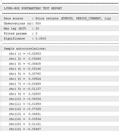
The report starts with a header block that shows exactly what was fed into the test: EURUSD price returns on PERIOD_CURRENT, using log returns, with 500 observations, a maximum lag of 20, no fitted-parameter adjustment (Fitted params = 0), and a significance level of 0.05. As before, I find this useful because it makes it easier to catch setup mistakes before interpreting the results — the wrong symbol, timeframe, or a leftover df adjustment would change what the test is actually telling me.

Below that, the script prints the sample autocorrelations from rho(1) through rho(20). None of them stand out on their own: they range roughly between -0.09 and +0.10, with the two largest in magnitude being rho(6) = 0.09524 and rho(18) = -0.09246, and rho(4) = -0.09146 close behind. Nothing here jumps off the page the way a strong pattern would.

This is where the Ljung-Box test earns its keep. Rather than judging each autocorrelation in isolation, it asks whether the group of autocorrelations up to a given lag is collectively large enough to reject the null hypothesis of no autocorrelation.

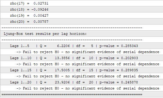
For this run, I tested the same four horizons as before:

• Lags 1–5: Q = 6.2206, df = 5, p = 0.285343 → fail to reject H0
• Lags 1–10: Q = 13.3856, df = 10, p = 0.202903 → fail to reject H0
• Lags 1–15: Q = 17.5005, df = 15, p = 0.289835 → fail to reject H0
• Lags 1–20: Q = 23.9206, df = 20, p = 0.245878 → fail to reject H0

Every one of the four horizons comes back well above the 0.05 threshold. Unlike a case where extending the horizon pushes the statistic into significant territory, here the p-value stays comfortably above 0.05 from lag 5 through lag 20. Adding further lags increases the Q statistic, but not enough relative to the corresponding increase in degrees of freedom to produce a statistically significant result.

A few observations from this particular run:

• No single horizon stands out. The p-values drift between roughly 0.20 and 0.29 across all four tests, with no horizon coming close to significance. This is a fairly clean "fail to reject" result across the board, not a borderline case sitting just above 0.05.
• The individual autocorrelations are modest and mixed in sign. rho(4), rho(6), and rho(18) are the largest in magnitude, but they don't share a consistent direction. The nearby lags do not show an obvious sustained positive or negative pattern that would, by itself, suggest a simple short-horizon momentum or mean-reversion structure. More importantly, the joint Ljung-Box tests do not provide statistically significant evidence of autocorrelation across any of the tested horizons.
• This is a "nothing found, for now" result, not proof of randomness. Failing to reject H0 at all four horizons means this test, on this 500-bar EURUSD sample, did not find statistically significant evidence of autocorrelation at the tested horizons. It doesn't prove the series is independent — a shorter-lived effect, a different timeframe, or a different sample period could still show something this test didn't pick up here.
• Timeframe context still matters even in a null result. Since this example was run on EURUSD H1, each lag represents one hour of observations, so lag 5 covers approximately five hours, lag 10 approximately ten hours, and so on. This is useful when deciding whether to extend the test further out or try a different set of horizons.
• The next step is the same regardless of the outcome. Whether the test comes back significant or not, the sensible move is to check whether the result holds on a different, non-overlapping sample rather than drawing a conclusion from one 500-bar window.

So, what did this particular run tell me? The EURUSD sample showed no statistically significant evidence of autocorrelation at any of the four tested horizons: lags 1–5, 1–10, 1–15, or 1–20. That's more informative than eyeballing the ACF values and guessing, but it is still evidence from a single 500-bar sample and from the specific autocorrelation structure tested here. Before drawing broader conclusions about the return series, I'd want to see whether the result holds across other sample periods, timeframes, or symbols.

Common Pitfalls

• Short samples. The chi-square approximation is asymptotic. With only a few dozen observations, p-values can be unreliable, and the (n − k) term in the Q formula becomes unstable as k approaches n. Treat results on small samples as indicative, not conclusive.
• Volatility clustering. Financial returns can have little or no autocorrelation in the mean while still showing strong clustering in volatility. The ordinary Ljung-Box test is aimed at autocorrelation in the series you give it, so it does not automatically diagnose every kind of volatility dependence. If you're working with a volatility model, it can make sense to test appropriately standardized residuals for any autocorrelation left over. If you specifically want to investigate volatility clustering, you can also look at squared residuals or use a test designed for ARCH effects.
  
• Multiple testing. If you test many lag sets, many symbols, or many parameter combinations and only report the one that came back significant, you've inflated your false-positive risk. InpLagSet can print several related horizon tests in one run, but comparing each p-value with alpha = 0.05 does not give the entire collection a 5% false-positive rate. The horizons overlap, so the tests are not independent, but the family of results still needs to be interpreted as multiple hypothesis tests. Decide on your lag horizons and significance level before looking at the results, and if the collection of tests is being used for a formal inference, consider an appropriate multiple-testing procedure or clearly treat the results as exploratory.

Conclusion

LjungBoxToolkit.mq5 gives me a way to test for serial dependence directly instead of relying on how a return series looks on a chart. I can run the same calculation on price returns, closed-deal results, or residuals exported from another model, and get the Q statistic, degrees of freedom, p-value, and test decision in the Experts tab.

The important part is what happens after the test. A significant result tells me that there is evidence of autocorrelation worth investigating. It does not tell me that I have found a profitable strategy. A non-significant result does not prove that the series is completely random either. The test gives me a statistical starting point, and the next step is to check whether the finding survives on other data.