Neural Networks in Trading: Memory Augmented Context-Aware Learning for Cryptocurrency Markets (Final Part)

Introduction

In the previous article, we introduced the MacroHFT framework, developed for high-frequency cryptocurrency trading (HFT). This framework represents a modern approach, combining context-dependent reinforcement learning methods with memory utilization, enabling efficient adaptation to dynamic market conditions while minimizing risks.

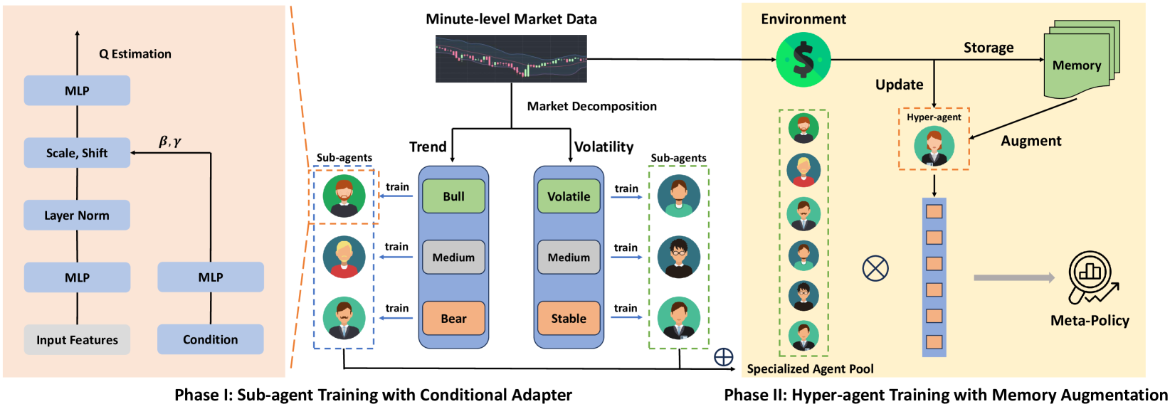
The operation principle of MacroHFT is based on two stages of training its individual components. In the first stage, market states are classified according to trend direction and volatility level. This process allows for the identification of key market states, which are then used to train specialized sub-agents. Each sub-agent is optimized to operate under specific scenarios. In the second stage, a hyper-agent equipped with a memory module is trained to coordinate the sub-agents' work. This module accounts for historical data, enabling more precise decisions based on prior experience.

The MacroHFT architecture includes several key components. The first is the data preprocessing module, which performs filtering and normalization of incoming market information. This eliminates noise and improves data quality, which is critically important for subsequent analysis.

Sub-agents are deep learning models trained on specific market scenarios. They use reinforcement learning methods to adapt to complex and rapidly changing conditions. The final component is the memory-augmented hyper-agent. It integrates the sub-agents' output, analyzing both historical events and the current market state. This allows for high predictive accuracy and resilience against market spikes.

Integrating all these components enables MacroHFT not only to function effectively under highly volatile market conditions but also to significantly improve profitability metrics. 

The original visualization of the MacroHFT framework is provided below.

In the practical section of the previous article, we created a hyper-agent object and implemented its interaction algorithm with sub-agents. Today, we will continue this work, focusing on new aspects of the MacroHFT architecture.

Risk Management Module

In the previous article, we organized the hyper-agent's operation as a CNeuronMacroHFTHyperAgent object and developed algorithms for its interaction with sub-agents. Additionally, we decided to use previously created analyst agents with more complex architectures as sub-agents. At first glance, this seems enough for implementing the MacroHFT framework. However, the current implementation has certain limitations: both the sub-agents and the hyper-agent analyze only the state of the environment. While this allows forecasting future price movements, determining trade direction, and setting stop loss and take profit levels, it does not address trade sizing, which is a critical element of the overall strategy.

Simply using a fixed trade size or calculating volume based on a fixed risk level relative to a projected stop-loss and account balance is possible. However, each forecast inherently carries an individual confidence level. It is logical to assume that this confidence level should play a central role in determining trade size. High confidence in a forecast permits larger trades, maximizing overall profitability, while low confidence suggests a more conservative approach.

Considering these factors, I decided to enhance the implementation with a risk management module. This module will be integrated into the existing architecture to provide a flexible, adaptive approach to trade sizing. Introducing risk management will improve the model's resilience to unstable market conditions, which is especially important in high-frequency trading.

It is important to note that, in this case, the risk management algorithm is partially "detached" from direct environmental analysis. Instead, the focus is on evaluating the impact of the agent's actions on financial results. The idea is to correlate each trade with changes in account balance and identify patterns indicating policy effectiveness. A growing number of profitable trades combined with a steadily increasing balance will indicate the success of the current policy, justifying higher risk per trade. Conversely, an increase in losing trades signals the need for a more conservative strategy to mitigate risk. This approach not only improves adaptation to changing market conditions but also enhances overall capital management efficiency. Additionally, to improve analysis quality, several account state projections will be created, each representing different aspects of its current and historical condition. This will allow for more precise evaluation of strategy performance and enable timely adaptation to market dynamics.

The risk management algorithm is implemented within the CNeuronMacroHFTvsRiskManager object, its structure is shown below.

class CNeuronMacroHFTvsRiskManager  :  public CResidualConv
  {
protected:
   CNeuronBaseOCL       caAccountProjection[2];
   CNeuronMemoryDistil  cMemoryAccount;
   CNeuronMemoryDistil  cMemoryAction;
   CNeuronRelativeCrossAttention cCrossAttention;
   //---
   virtual bool      feedForward(CNeuronBaseOCL *NeuronOCL) override { return false; }
   virtual bool      feedForward(CNeuronBaseOCL *NeuronOCL, CBufferFloat *SecondInput) override;
   virtual bool      calcInputGradients(CNeuronBaseOCL *NeuronOCL) override { return false; }
   virtual bool      calcInputGradients(CNeuronBaseOCL *NeuronOCL, CBufferFloat *SecondInput,
                       CBufferFloat *SecondGradient, ENUM_ACTIVATION SecondActivation = None) override;
   virtual bool      updateInputWeights(CNeuronBaseOCL *NeuronOCL) override { return false; }
   virtual bool      updateInputWeights(CNeuronBaseOCL *NeuronOCL, CBufferFloat *SecondInput) override;

public:
                     CNeuronMacroHFTvsRiskManager(void) {};
                    ~CNeuronMacroHFTvsRiskManager(void) {};
   //---
   virtual bool      Init(uint numOutputs, uint myIndex, COpenCLMy *open_cl,
                          uint window, uint window_key, uint units_count, uint heads,
                          uint stack_size, uint nactions, uint account_decr,
                          ENUM_OPTIMIZATION optimization_type, uint batch);
   //---
   virtual int       Type(void) override   const   {  return defNeuronMacroHFTvsRiskManager; }
   //---
   virtual bool      Save(const int file_handle) override;
   virtual bool      Load(const int file_handle) override;
   //---
   virtual bool      WeightsUpdate(CNeuronBaseOCL *source, float tau) override;
   virtual void      SetOpenCL(COpenCLMy *obj) override;
   //---
   virtual bool      Clear(void) override;
  }; 

In the presented structure, one can observe a standard set of overridable methods and several internal objects that play a key role in the implementation of the risk management mechanism described above. The functionality of these internal objects will be discussed in detail when describing the class methods, providing a deeper understanding of their usage logic.

All internal objects in our risk management class are declared as static, simplifying the object structure. This allows the constructor and destructor to remain empty, as no additional operations are required for initialization or memory cleanup. Initialization of all inherited and declared objects is performed in the Init method, responsible for setting up the class architecture upon creation.

The class parameters include constants that enable unambiguous interpretation of the object's architecture.

bool CNeuronMacroHFTvsRiskManager::Init(uint numOutputs, uint myIndex, COpenCLMy *open_cl,
                                        uint window, uint window_key, uint units_count, uint heads,
                                        uint stack_size, uint nactions, uint account_decr,
                                        ENUM_OPTIMIZATION optimization_type, uint batch)
  {
   if(!CResidualConv::Init(numOutputs, myIndex, open_cl, 3, 3, (nactions + 2) / 3, optimization_type, batch))
      return false;

Within the method body, the parent class method of the same name is immediately called. In this case, it is a convolutional block with feedback. It is important to note that the expected output of this module is a tensor representing a trade decision matrix. Each row describes a separate trade and contains a vector of trade parameters: volume, stop loss, and take profit. To organize trade analysis correctly, buy and sell trades are treated as separate rows, allowing independent analysis of each trade.

When organizing convolutional operations, the kernel size and stride are set to 3, corresponding to the number of parameters in the trade description.

Next, let's view the initialization process of internal objects. It is important to note that the risk management module relies on two key data sources: agent actions and a vector describing the analyzed account state. The main data stream, representing agent actions, is provided as a neural layer object. The secondary stream, containing the account state description, is passed through a data buffer.

For proper functioning of all internal components, both data streams must be represented as neural layer objects. Therefore, the first step is initializing a fully connected neural layer, into which data from the second stream will be transferred.

   int index = 0;
   if(!caAccountProjection[0].Init(0, index, OpenCL, account_decr, optimization, iBatch))
      return false;

The next stage adds a fully connected layer designed to form projections of the account state description. This trainable layer generates a tensor containing multiple projections of the analyzed account state in subspaces of specified dimensionality. The number of projections and the dimensionality of subspaces are provided as method parameters, allowing flexible layer configuration for various tasks.

   index++;
   if(!caAccountProjection[1].Init(0, index, OpenCL, window * units_count, optimization, iBatch))
      return false;

The raw data received by the risk management module provides only a static description of the analyzed state. However, to accurately evaluate the agent's policy effectiveness, dynamic changes must be considered. Memory modules are applied to both information streams, capturing the temporal sequence of data. A key decision is whether to store the original account state vector or its projections. The original vector is smaller and more resource-efficient, while projections generated after memory processing provide richer information by incorporating account balance dynamics into the static data.

   index++;
   if(!cMemoryAccount.Init(caAccountProjection[1].Neurons(), index, OpenCL, account_decr,
                           window_key, 1, heads, stack_size, optimization, iBatch))
      return false;

The memory module for agent trades operates at the level of individual trades.

   index++;
   if(!cMemoryAction.Init(0, index, OpenCL, 3, window_key, (nactions + 2) / 3,
                          heads, stack_size, optimization, iBatch))
      return false;

For more effective policy analysis, a cross-attention module is employed. This module correlates recent agent actions with account state dynamics, identifying the relationship between decisions and resulting financial results.

   index++;
   if(!cCrossAttention.Init(0, index, OpenCL, 3, window_key, (nactions + 2) / 3,
                            heads, window, units_count, optimization, iBatch))
      return false;
//---
   return true;
  }

At this point, the initialization of internal objects is complete. The entire method also completes here. We just need to return the logical result of the operations to the calling program.

After initializing the risk management object, we proceed to constructing the feed-forward pass algorithm in the feedForward method.

bool CNeuronMacroHFTvsRiskManager::feedForward(CNeuronBaseOCL *NeuronOCL, CBufferFloat *SecondInput)
  {
   if(caAccountProjection[0].getOutput() != SecondInput)
     {
      if(!caAccountProjection[0].SetOutput(SecondInput, true))
         return false;
     }

The method receives pointers to two raw data objects. One is provided as a data buffer, whose contents must be transferred to an internal neural layer object. Instead of copying all data, I use a more efficient approach: the internal object's buffer pointer is replaced with the pointer to the input data buffer. This significantly accelerates processing.

Next, both information streams are enriched with additional data on accumulated dynamics. The data is passed through specialized memory modules that capture past states and changes, enabling temporal dependencies to be preserved and maintaining context for more accurate processing.

   if(!cMemoryAccount.FeedForward(caAccountProjection[0].AsObject()))
      return false;
   if(!cMemoryAction.FeedForward(NeuronOCL))
      return false;

Based on these enriched data, projections of the account state vector are generated. These projections provide a comprehensive basis for analyzing account dynamics and assessing the impact of past actions on the current state.

   if(!caAccountProjection[1].FeedForward(cMemoryAccount.AsObject()))
      return false;

Once the preliminary data processing stage is complete, the agent's policy impact on financial outcomes is analyzed using the cross-attention block. By correlating agent actions with financial changes, the relationship between decisions and outcomes is revealed.

   if(!cCrossAttention.FeedForward(cMemoryAction.AsObject(), caAccountProjection[1].getOutput()))
      return false;

The final "touch" in forming the trading decision is provided by parent class mechanisms, which perform the ultimate information processing.

   return CResidualConv::feedForward(cCrossAttention.AsObject());
  }

The logical result of these operations is returned to the calling program, and the method concludes.

The backpropagation methods employ linear algorithms and are unlikely to require additional explanation during independent study. With this, the review of the risk management object is complete. The full code of the class and all its methods is provided in the attachment.

Model Architecture

We continue our work on implementing the approaches of the MacroHFT framework using MQL5. The next stage involves building the architecture of the trainable model. In this case, we will train a single Actor model, whose architecture is defined in the CreateDescriptions method.

bool CreateDescriptions(CArrayObj *&actor)
  {
//---
   CLayerDescription *descr;
//---
   if(!actor)
     {
      actor = new CArrayObj();
      if(!actor)
         return false;
     }

The method receives a pointer to a dynamic array object for recording the architecture of the model being created. And in the method body, we immediately check the relevance of the received pointer. If necessary, we create a new instance of the dynamic array object.

Next, we create a description of a fully connected layer, which, in this case, is used to receive the raw input data and must have sufficient size to accommodate the tensor describing the analyzed environmental state.

//--- Actor
   actor.Clear();
//--- Input layer
   if(!(descr = new CLayerDescription()))
      return false;
   descr.type = defNeuronBaseOCL;
   int prev_count = descr.count = (HistoryBars * BarDescr);
   descr.activation = None;
   descr.optimization = ADAM;
   if(!actor.Add(descr))
     {
      delete descr;
      return false;
     }

It is important to remind that the raw input data is obtained directly from the terminal. The preprocessing block for these data is organized as a batch normalization layer.

//--- layer 1
   if(!(descr = new CLayerDescription()))
      return false;
   descr.type = defNeuronBatchNormOCL;
   descr.count = prev_count;
   descr.batch = 1e4;
   descr.activation = None;
   descr.optimization = ADAM;
   if(!actor.Add(descr))
     {
      delete descr;
      return false;
     }

After normalization, the environmental state description is passed to the layer we created within the MacroHFT framework.

//--- layer 2
   if(!(descr = new CLayerDescription()))
      return false;
   descr.type = defNeuronMacroHFT;
//--- Windows
     {
      int temp[] = {BarDescr, 120, NActions}; //Window, Stack Size, N Actions
      if(ArrayCopy(descr.windows, temp) < int(temp.Size()))
         return false;
     }
   descr.count = HistoryBars;
   descr.window_out = 32;
   descr.step = 4;                              // Heads
   descr.layers =3;
   descr.batch = 1e4;
   descr.activation = None;
   descr.optimization = ADAM;
   if(!actor.Add(descr))
     {
      delete descr;
      return false;
     }

Note that MacroHFT is designed to operate on the 1-minute timeframe. Accordingly, the memory stack of environmental states has been increased to 120 elements, corresponding to a 2-hour sequence. This allows for more comprehensive accounting of market dynamics, enabling more accurate forecasting and decision-making within the trading strategy.

As previously mentioned, this module focuses exclusively on analyzing the environmental state and does not provide risk assessment capabilities. Therefore, the next step is to add a risk management module.

//--- layer 3
   if(!(descr = new CLayerDescription()))
      return false;
   descr.type = defNeuronMacroHFTvsRiskManager;
//--- Windows
     {
      int temp[] = {3, 15, NActions,AccountDescr}; //Window, Stack Size, N Actions, Account Description
      if(ArrayCopy(descr.windows, temp) < int(temp.Size()))
         return false;
     }
   descr.count = 10;
   descr.window_out = 16;
   descr.step = 4;                              // Heads
   descr.batch = 1e4;
   descr.activation = None;
   descr.optimization = ADAM;
   if(!actor.Add(descr))
     {
      delete descr;
      return false;
     }

In this case, we reduce the memory stack to 15 elements, which decreases the amount of data processed and allows focus on shorter-term dynamics. This ensures a faster reaction to market changes.

The output of the risk management module is normalized values. To map them into the action space required by the Agent, we use a convolutional layer with an appropriate activation function.

//--- layer 4
   if(!(descr = new CLayerDescription()))
      return false;
   descr.type = defNeuronConvSAMOCL;
   descr.count = NActions / 3;
   descr.window = 3;
   descr.step = 3;
   descr.window_out = 3;
   descr.activation = SIGMOID;
   descr.optimization = ADAM;
   descr.probability = Rho;
   if(!actor.Add(descr))
     {
      delete descr;
      return false;
     }
//---
   return true;
  }

Upon completing the method, the logical result of the operations is returned to the calling program.

Note that in this implementation, we do not use a stochastic head for the agent. In my view, in high-frequency trading, its use would only introduce unnecessary noise. In HFT strategies, it is crucial to minimize random factors to ensure fast and well-founded reactions to market changes.

Training the Model

At this stage, we have completed the implementation of our interpretation of the approaches proposed by the MacroHFT framework authors using MQL5. The architecture of the trainable model has been defined. It is now time to train the model. First, however, we need to collect a training dataset. Previously, models were trained using hourly timeframe data. In this case, we require information from the 1-minute timeframe.

It is important to note that reducing the timeframe increases the data volume. Clearly, the same historical interval produces 60 times more bars. This leads to a proportional increase in the training dataset size if all other parameters remain the same. Measures must therefore be taken to reduce it. There are two approaches: shorten the training period or reduce the number of passes stored in the training dataset.

We decided to maintain a one-year training period, which, in my opinion, is the minimum interval that allows at least some insight into seasonality. However, the length of each pass was limited to one month. For each month, two passes of random policies were saved, resulting in a total of 24 passes. While this is insufficient for full training, this format already produces a training dataset file exceeding 3 GB.

These constraints for collecting the training dataset were quite strict. It should be noted that no one expects profitable results from random agent policies. Unsurprisingly, we quickly lost the entire deposit during all passes. To prevent testing from stopping due to margin calls, we set a minimum account balance threshold for generating trading decisions. This allowed us to retain all environmental states in the dataset for the analyzed period, albeit without rewards for trades.

It is also worth noting that the MacroHFT authors used their own list of technical indicators when training their cryptocurrency trading model. This list can be found in the appendix of the original article.

We chose to retain the previously used list of analyzed indicators. This allows a direct comparison of the effectiveness of the implemented solution with previously built and trained models. Using the same indicators ensures an objective evaluation, directly comparing results to identify the strengths and weaknesses of the new model.

Data collection for the training dataset is performed by the Expert Advisor "...\MacroHFT\Research.mq5". For this article, we will focus on the OnTick method, where the core algorithm for obtaining terminal data and executing trades is implemented.

void OnTick()
  {
//---
   if(!IsNewBar())
      return;

Within the method body, we first check for the opening of a new bar. Only then are further operations executed. Initially, we update the analyzed technical indicator data and load historical price movement data.

   int bars = CopyRates(Symb.Name(), TimeFrame, iTime(Symb.Name(), TimeFrame, 1), HistoryBars, Rates);
   if(!ArraySetAsSeries(Rates, true))
      return;
//---
   RSI.Refresh();
   CCI.Refresh();
   ATR.Refresh();
   MACD.Refresh();
   Symb.Refresh();
   Symb.RefreshRates();

Next, we organize a loop that forms the buffer describing the environmental state based on data received from the terminal.

   float atr = 0;
   for(int b = 0; b < (int)HistoryBars; b++)
     {
      float open = (float)Rates[b].open;
      float rsi = (float)RSI.Main(b);
      float cci = (float)CCI.Main(b);
      atr = (float)ATR.Main(b);
      float macd = (float)MACD.Main(b);
      float sign = (float)MACD.Signal(b);
      if(rsi == EMPTY_VALUE || cci == EMPTY_VALUE || atr == EMPTY_VALUE ||
                               macd == EMPTY_VALUE || sign == EMPTY_VALUE)
         continue;
      //---
      int shift = b * BarDescr;
      sState.state[shift] = (float)(Rates[b].close - open);
      sState.state[shift + 1] = (float)(Rates[b].high - open);
      sState.state[shift + 2] = (float)(Rates[b].low - open);
      sState.state[shift + 3] = (float)(Rates[b].tick_volume / 1000.0f);
      sState.state[shift + 4] = rsi;
      sState.state[shift + 5] = cci;
      sState.state[shift + 6] = atr;
      sState.state[shift + 7] = macd;
      sState.state[shift + 8] = sign;
     }
   bState.AssignArray(sState.state);

It should be noted that oscillator values have a comparable appearance and maintain distribution stability over time. To achieve this, only deviations between price movement indicators are analyzed, preserving distribution stability and avoiding excessive fluctuations that could distort analysis results.

The next step is creating the account state description vector, considering open positions and financial outcomes achieved. First, we collect information on open positions.

   sState.account[0] = (float)AccountInfoDouble(ACCOUNT_BALANCE);
   sState.account[1] = (float)AccountInfoDouble(ACCOUNT_EQUITY);
//---
   double buy_value = 0, sell_value = 0, buy_profit = 0, sell_profit = 0;
   double position_discount = 0;
   double multiplyer = 1.0 / (60.0 * 60.0 * 10.0);
   int total = PositionsTotal();
   datetime current = TimeCurrent();
   for(int i = 0; i < total; i++)
     {
      if(PositionGetSymbol(i) != Symb.Name())
         continue;
      double profit = PositionGetDouble(POSITION_PROFIT);
      switch((int)PositionGetInteger(POSITION_TYPE))
        {
         case POSITION_TYPE_BUY:
            buy_value += PositionGetDouble(POSITION_VOLUME);
            buy_profit += profit;
            break;
         case POSITION_TYPE_SELL:
            sell_value += PositionGetDouble(POSITION_VOLUME);
            sell_profit += profit;
            break;
        }
      position_discount += profit - (current - PositionGetInteger(POSITION_TIME)) * 
                                                      multiplyer * MathAbs(profit);
     }
   sState.account[2] = (float)buy_value;
   sState.account[3] = (float)sell_value;
   sState.account[4] = (float)buy_profit;
   sState.account[5] = (float)sell_profit;
   sState.account[6] = (float)position_discount;
   sState.account[7] = (float)Rates[0].time;

We then generate harmonics of the timestamp.

   bTime.Clear();
   double time = (double)Rates[0].time;
   double x = time / (double)(D'2024.01.01' - D'2023.01.01');
   bTime.Add((float)MathSin(x != 0 ? 2.0 * M_PI * x : 0));
   x = time / (double)PeriodSeconds(PERIOD_MN1);
   bTime.Add((float)MathCos(x != 0 ? 2.0 * M_PI * x : 0));
   x = time / (double)PeriodSeconds(PERIOD_W1);
   bTime.Add((float)MathSin(x != 0 ? 2.0 * M_PI * x : 0));
   x = time / (double)PeriodSeconds(PERIOD_D1);
   bTime.Add((float)MathSin(x != 0 ? 2.0 * M_PI * x : 0));
   if(bTime.GetIndex() >= 0)
      bTime.BufferWrite();

Only after completing the preparatory work do we consolidate all financial results into a single data buffer.

   bAccount.Clear();
   bAccount.Add((float)((sState.account[0] - PrevBalance) / PrevBalance));
   bAccount.Add((float)(sState.account[1] / PrevBalance));
   bAccount.Add((float)((sState.account[1] - PrevEquity) / PrevEquity));
   bAccount.Add(sState.account[2]);
   bAccount.Add(sState.account[3]);
   bAccount.Add((float)(sState.account[4] / PrevBalance));
   bAccount.Add((float)(sState.account[5] / PrevBalance));
   bAccount.Add((float)(sState.account[6] / PrevBalance));
   bAccount.AddArray(GetPointer(bTime));
//---
   if(bAccount.GetIndex() >= 0)
      if(!bAccount.BufferWrite())
         return;

With all required raw data prepared, we check the account balance. If sufficient, the model performs a feed-forward pass.

   double min_lot = Symb.LotsMin();
   double step_lot = Symb.LotsStep();
   double stops = MathMax(Symb.StopsLevel(), 1) * Symb.Point();
//---
   vector<float> temp;
   if(sState.account[0] > 50)
     {
      if(!Actor.feedForward((CBufferFloat*)GetPointer(bState), 1, false, GetPointer(bAccount)))
        {
         PrintFormat("%s -> %d", __FUNCTION__, __LINE__);
         return;
        }
      Actor.getResults(temp);
      if(temp.Size() < NActions)
         temp = vector<float>::Zeros(NActions);
      //---
      for(int i = 0; i < NActions; i++)
        {
         float random = float(rand() / 32767.0 * 5 * min_lot - min_lot);
         temp[i] += random;
        }
     }
   else
      temp = vector<float>::Zeros(NActions);

To increase environmental exploration, a small amount of noise is added to the generated trading decision. While seemingly unnecessary during random policy execution in the initial stage, it proves useful when updating the training dataset using a pre-trained policy.

If the account balance reaches the lower limit, the trade decision vector is filled with zeros, indicating no trades.

Next, we work with the obtained trade decision vector. Initially, volumes of counter operations are excluded.

   PrevBalance = sState.account[0];
   PrevEquity = sState.account[1];
//---
   if(temp[0] >= temp[3])
     {
      temp[0] -= temp[3];
      temp[3] = 0;
     }
   else
     {
      temp[3] -= temp[0];
      temp[0] = 0;
     }

We then check the parameters of the long position. If a long position is not specified by the trading decision, we check for and close any previously opened long positions.

//--- buy control
   if(temp[0] < min_lot || (temp[1] * MaxTP * Symb.Point()) <= stops || 
                             (temp[2] * MaxSL * Symb.Point()) <= stops)
     {
      if(buy_value > 0)
         CloseByDirection(POSITION_TYPE_BUY);
     }

If opening or holding a long position is necessary, we first bring the trade parameters into the required format and adjust the trading levels of already open positions.

   else
     {
      double buy_lot = min_lot + MathRound((double)(temp[0] - min_lot) / step_lot) * step_lot;
      double buy_tp = NormalizeDouble(Symb.Ask() + temp[1] * MaxTP * Symb.Point(), Symb.Digits());
      double buy_sl = NormalizeDouble(Symb.Ask() - temp[2] * MaxSL * Symb.Point(), Symb.Digits());
      if(buy_value > 0)
         TrailPosition(POSITION_TYPE_BUY, buy_sl, buy_tp);

We then adjust the volume of open positions through scaling up or partial closure.

      if(buy_value != buy_lot)
        {
         if(buy_value > buy_lot)
            ClosePartial(POSITION_TYPE_BUY, buy_value - buy_lot);
         else
            Trade.Buy(buy_lot - buy_value, Symb.Name(), Symb.Ask(), buy_sl, buy_tp);
        }
     }

The parameters of short positions are handled in a similar manner.

//--- sell control
   if(temp[3] < min_lot || (temp[4] * MaxTP * Symb.Point()) <= stops || 
                              (temp[5] * MaxSL * Symb.Point()) <= stops)
     {
      if(sell_value > 0)
         CloseByDirection(POSITION_TYPE_SELL);
     }
   else
     {
      double sell_lot = min_lot + MathRound((double)(temp[3] - min_lot) / step_lot) * step_lot;;
      double sell_tp = NormalizeDouble(Symb.Bid() - temp[4] * MaxTP * Symb.Point(), Symb.Digits());
      double sell_sl = NormalizeDouble(Symb.Bid() + temp[5] * MaxSL * Symb.Point(), Symb.Digits());
      if(sell_value > 0)
         TrailPosition(POSITION_TYPE_SELL, sell_sl, sell_tp);
      if(sell_value != sell_lot)
        {
         if(sell_value > sell_lot)
            ClosePartial(POSITION_TYPE_SELL, sell_value - sell_lot);
         else
            Trade.Sell(sell_lot - sell_value, Symb.Name(), Symb.Bid(), sell_sl, sell_tp);
        }
     }

After executing the trades, a reward vector is generated.

   sState.rewards[0] = bAccount[0];
   sState.rewards[1] = 1.0f - bAccount[1];
   if((buy_value + sell_value) == 0)
      sState.rewards[2] -= (float)(atr / PrevBalance);
   else
      sState.rewards[2] = 0;

All accumulated data is then transferred to the data storage buffer for the training dataset, and we wait for the event of a new bar opening.

   for(ulong i = 0; i < NActions; i++)
      sState.action[i] = temp[i];
   if(!Base.Add(sState))
      ExpertRemove();
  }

Note that if new data cannot be added to the training dataset buffer, the program is initialized to close. This can occur either due to an error or when the buffer becomes fully filled.

The complete code for this advisor is provided in the attachment.

The actual collection of the training dataset is performed in the MetaTrader 5 Strategy Tester via slow optimization.  

Clearly, a training dataset collected with a limited number of passes requires a special approach to model training. Especially considering that a significant portion of the data consists solely of environmental state information, which limits the learning potential. In such conditions, it seems optimal to train the model based on "nearly ideal" trading decisions. This method, which we used in training several recent models, allows the data to be used as efficiently as possible despite its limited size.

It is also worth noting that the model training program works exclusively with the training dataset and does not depend on the timeframe or financial instrument used for data collection. This provides a significant advantage, as the previously developed training program can be reused without modifying its algorithm. Thus, existing resources and methods can be leveraged efficiently, saving time and effort without compromising the quality of model training.

Test

We have completed extensive work implementing our interpretation of the approaches proposed by the MacroHFT framework authors using MQL5. The next step is to evaluate the effectiveness of the implemented methods on real historical data.

It should be noted that the implementation presented here differs significantly from the original, including in the choice of technical indicators. This will inevitably affect the results, so any conclusions are preliminary and specific to these modifications.

For model training, we used EURUSD data from 2024 on the 1-minute timeframe (M1). The analyzed indicator parameters were left unchanged to focus on evaluating the algorithms and approaches themselves, without confounding effects from indicator settings. The procedure for collecting the training dataset and training the model was described above.

The trained model was tested on historical data from January 2025. The test results are presented below.

It should be noted that over the two-week testing period, the model executed only eight trades, which is undoubtedly low for a high-frequency trading Expert Advisor. On the other hand, the efficiency of executed trades is notable — only one trade was unprofitable. This resulted in a profit factor of 2.47.

Upon detailed examination of the trade history, one can observe scaling up on the upward trend.

Conclusion

We explored the MacroHFT framework, which is an innovative and promising tool for high-frequency trading in cryptocurrency markets. A key feature of this framework is its ability to account for both macroeconomic contexts and local market dynamics. This combination allows for effective adaptation to rapidly changing financial conditions and more informed trading decisions.

In the practical part of our work, we implemented our interpretation of the proposed approaches using MQL5, making some adaptations to the framework's operation. We trained the model on real historical data and tested it on data outside the training set. While the number of trades executed was disappointing and does not reflect typical high-frequency trading. This may be attributed to the suboptimal choice of technical indicators or the limited training dataset. Verifying these assumptions requires further investigation. However, the test results demonstrated the model's ability to identify genuinely stable patterns, resulting in a high proportion of profitable trades on the test dataset.

References

• MacroHFT: Memory Augmented Context-aware Reinforcement Learning On High Frequency Trading
• Other articles from this series

Programs used in the article

#	Name	Type	Description
1	Research.mq5	Expert Advisor	Expert Advisor for collecting examples
2	ResearchRealORL.mq5	Expert Advisor	Expert Advisor for collecting samples using the Real-ORL method
3	Study.mq5	Expert Advisor	Model training Expert Advisor
4	Test.mq5	Expert Advisor	Model testing Expert Advisor
5	Trajectory.mqh	Class library	System state and model architecture description structure
6	NeuroNet.mqh	Class library	A library of classes for creating a neural network
7	NeuroNet.cl	Library	OpenCL program code