Neural Networks in Trading: Transformer with Relative Encoding

MetaTrader 5 — Trading systems | 26 May 2025, 13:35

1 801

Dmitriy Gizlyk

Introduction

Price forecasting and market trend prediction are central tasks for successful trading and risk management. High-quality price movement forecasts enable traders to make timely decisions and avoid financial losses. However, in highly volatile markets, traditional machine learning models may be limited in their capabilities.

Transitioning from training models from scratch to pretraining on large sets of unlabeled data, followed by fine-tuning for specific tasks, allows us to achieve high-accuracy forecasting without the need to collect massive volumes of new data. For example, models based on the Transformer architecture, adapted for financial data, can leverage information on asset correlations, temporal dependencies, and other factors to produce more accurate predictions. The implementation of alternative attention mechanisms helps account for key market dependencies, significantly enhancing model performance. This opens new opportunities for developing trading strategies while minimizing manual tuning and reliance on complex rule-based models.

One such alternative attention algorithm was introduced in the paper "Relative Molecule Self-Attention Transformer". The authors proposed a new Self-Attention formula for molecular graphs that meticulously processes various input features to achieve higher accuracy and reliability across many chemical domains. Relative Molecule Attention Transformer (R-MAT) is a pretrained model based on the Transformer architecture. It represents a novel variant of relative Self-Attention that effectively integrates distance and neighborhood information. R-MAT delivers state-of-the-art, competitive performance across a wide range of tasks.

1. The R-MAT Algorithm

In natural language processing, the vanilla Self-Attention layer does not account for the positional information of input tokens, that is, if the input data is rearranged, the result will remain unchanged. To incorporate positional information into the input data, the vanilla Transformer enriches it with absolute position encoding. In contrast, relative position encoding introduces the relative distance between each pair of tokens, leading to substantial improvements in certain tasks. The R-MAT algorithm employs relative token position encoding.

The core idea is to enhance the flexibility of processing information about graphs and distances. The authors of the R-MAT method adapted relative position encoding to enrich the Self-Attention block with an efficient representation of the relative positions of elements in the input sequence.

The mutual positioning of two atoms in a molecule is characterized by three interrelated factors:

their relative distance,
their distance in the molecular graph,
their physicochemical relationship.

Two atoms are represented by vectors 𝒙i and 𝒙j of dimension D. The authors propose encoding their relationship using an atom pair embedding 𝒃ij of dimension D′. This embedding is then used in the Self-Attention module after the projection layer.

The process begins by encoding the neighborhood order between two atoms with information about how many other nodes are located between nodes i and j in the original molecular graph. This is followed by radial basis distance encoding. Finally, each bond is highlighted to reflect the physicochemical relationship between atom pairs.

The authors note that, while these features can be easily learned during pretraining, such construction can be highly beneficial for training R-MAT on smaller datasets.

The resulting token 𝒃ij for each atom pair in the molecule is used to define a new Self-Attention layer, which the authors termed Relative Molecule Self-Attention.

In this new architecture, the authors mirror the Query-Key-Value design of vanilla Self-Attention. The token 𝒃ij is transformed into key- and value-specific vectors 𝒃ijV and 𝒃ijK using two neural networks φV and φK. Each neural network consists of two layers. These include a hidden layer shared across all attention heads and an output layer that creates distinct relative embeddings for different attention heads. Relative Self-Attention can be expressed as follows:

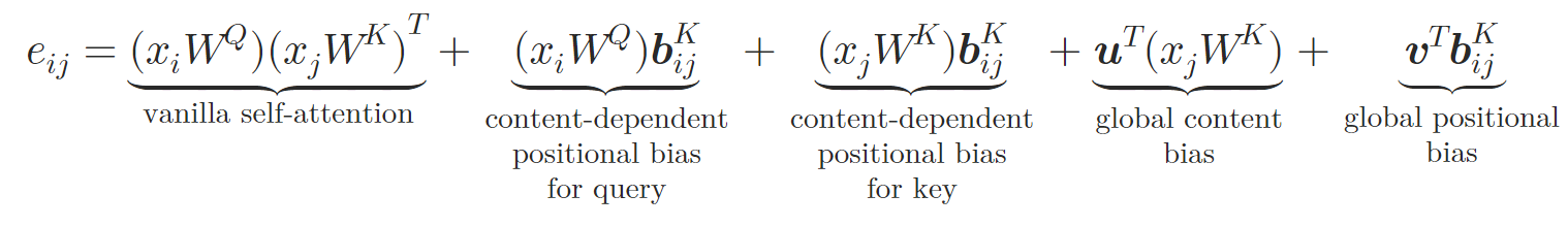
where 𝒖 and 𝒗 are learnable vectors.

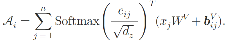
In this way, the authors enrich the Self-Attention block by embedding atomic relationships. During the computation of attention weights, they introduce a content-dependent positional bias, a global context bias, and a global positional bias, all calculated based on 𝒃ijK. Then, during the calculation of the weighted average attention, the authors also incorporate information from the alternative embedding 𝒃ijV.

The Relative Self-Attention block is used to construct the Relative Molecule Attention Transformer (R-MAT).

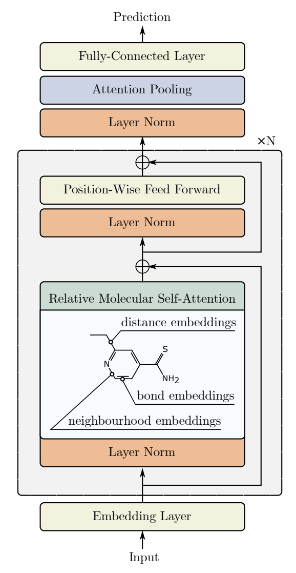
The input data is presented as a matrix of size Natoms×36, which is processed by a stack of N layers of Relative Molecule Self-Attention. Each attention layer is followed by an MLP with residual connections, similar to the vanilla Transformer model.

After processing the input data through the attention layers, the authors aggregate the representation into a fixed-size vector. Self-Attention pooling is used for this purpose.

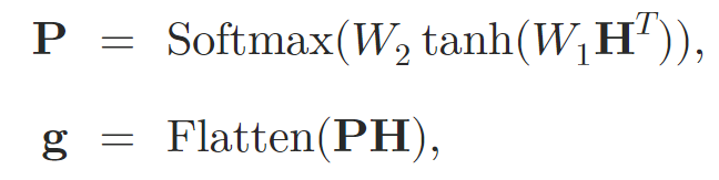
where 𝐇 denotes the hidden state obtained from the Self-Attention layers, and W1 and W2 are the attention pooling weights.

The graph embedding 𝐠 is then fed into a two-level MLP with the leaky-ReLU activation function, which outputs the final prediction.

The author's visualization of the method is presented below.

2. Implementation in MQL5

After examining the theoretical aspects of the proposed Relative Molecule Attention Transformer (R-MAT) method, we move on to developing our own interpretation of the proposed approaches using MQL5. Right away, I should mention that I have decided to divide the construction of the proposed algorithm into separate modules. We will first create a dedicated object for implementing the relative Self-Attention algorithm, and then assemble the R-MAT model into a separate high-level class.

2.1 Relative Self-Attention Module

As you know, we have offloaded the majority of the computations to the OpenCL context. Consequently, as we begin implementing the new algorithm, we need to add the missing kernels to our OpenCL program. The first kernel we will create is the feed-forward kernel MHRelativeAttentionOut. Although this kernel is based on previously discussed implementations of the Self-Attention algorithm, here we have a significant increase in the number of global buffers, whose purposes we will explore as we construct the algorithm.

__kernel void MHRelativeAttentionOut(__global const float *q,         ///<[in] Matrix of Querys
                                     __global const float *k,         ///<[in] Matrix of Keys
                                     __global const float *v,         ///<[in] Matrix of Values
                                     __global const float *bk,        ///<[in] Matrix of Positional Bias Keys
                                     __global const float *bv,        ///<[in] Matrix of Positional Bias Values
                                     __global const float *gc,        ///<[in] Global content bias vector
                                     __global const float *gp,        ///<[in] Global positional bias vector
                                     __global float *score,           ///<[out] Matrix of Scores
                                     __global float *out,             ///<[out] Matrix of attention
                                     const int dimension              ///< Dimension of Key
                                    )
  {
//--- init
   const int q_id = get_global_id(0);
   const int k_id = get_global_id(1);
   const int h = get_global_id(2);
   const int qunits = get_global_size(0);
   const int kunits = get_global_size(1);
   const int heads = get_global_size(2);

This kernel is designed to operate within a three-dimensional task space, where each dimension corresponds to Query, Key, and Heads. Within the second dimension, we create workgroups.

Inside the kernel body, we immediately identify the current thread across all dimensions of the task space, as well as determine its boundaries. We then define constant offsets in the data buffers to access the necessary elements.

   const int shift_q = dimension * (q_id * heads + h);
   const int shift_kv = dimension * (heads * k_id + h);
   const int shift_gc = dimension * h;
   const int shift_s = kunits * (q_id *  heads + h) + k_id;
   const int shift_pb = q_id * kunits + k_id;
   const uint ls = min((uint)get_local_size(1), (uint)LOCAL_ARRAY_SIZE);
   float koef = sqrt((float)dimension);
   if(koef < 1)
      koef = 1;

Then we create an array in local memory for exchanging information within the workgroup.

   __local float temp[LOCAL_ARRAY_SIZE];

Next, in accordance with the relative Self-Attention algorithm, we need to calculate the attention coefficients. To achieve this, we compute the dot product of several vectors and sum the resulting values. Here, we use the fact that the dimensions of all the multiplied vectors are the same. Consequently, a single loop is sufficient to perform the necessary multiplications of all the vectors.

//--- score
   float sc = 0;
   for(int d = 0; d < dimension; d++)
     {
      float val_q = q[shift_q + d];
      float val_k = k[shift_kv + d];
      float val_bk = bk[shift_kv + d];
      sc += val_q * val_k + 
	    val_q * val_bk + 
            val_k * val_bk + 
            gc[shift_q + d] * val_k + 
            gp[shift_q + d] * val_bk;
     }

The next step involves normalizing the computed attention coefficients across individual Queries. For normalization, we use the Softmax function, just as in the vanilla algorithm. Thus, the normalization procedure is carried over from our existing implementations without any modifications. In this step, we first compute the exponential value of the coefficient.

   sc = exp(sc / koef);
   if(isnan(sc) || isinf(sc))
      sc = 0;

Then we sum up the obtained coefficients within the working group using the array created earlier in local memory.

//--- sum of exp
   for(int cur_k = 0; cur_k < kunits; cur_k += ls)
     {
      if(k_id >= cur_k && k_id < (cur_k + ls))
        {
         int shift_local = k_id % ls;
         temp[shift_local] = (cur_k == 0 ? 0 : temp[shift_local]) + sc;
        }
      barrier(CLK_LOCAL_MEM_FENCE);
     }
   uint count = min(ls, (uint)kunits);
//---
   do
     {
      count = (count + 1) / 2;
      if(k_id < ls)
         temp[k_id] += (k_id < count && (k_id + count) < kunits ? temp[k_id + count] : 0);
      if(k_id + count < ls)
         temp[k_id + count] = 0;
      barrier(CLK_LOCAL_MEM_FENCE);
     }
   while(count > 1);

Now we can divide the previously obtained coefficient by the total sum and save the normalized value into the corresponding global buffer.

//--- score
   float sum = temp[0];
   if(isnan(sum) || isinf(sum) || sum <= 1e-6f)
      sum = 1;
   sc /= sum;
   score[shift_s] = sc;
   barrier(CLK_LOCAL_MEM_FENCE);

After computing the normalized dependence coefficients, we can compute the result of the attention operation. The algorithm here is very close to vanilla. We just add the summation of vectors Value and bijV before multiplying by the attention factor.

//--- out
   for(int d = 0; d < dimension; d++)
     {
      float val_v = v[shift_kv + d];
      float val_bv = bv[shift_kv + d];
      float val = sc * (val_v + val_bv);
      if(isnan(val) || isinf(val))
         val = 0;
      //--- sum of value
      for(int cur_v = 0; cur_v < kunits; cur_v += ls)
        {
         if(k_id >= cur_v && k_id < (cur_v + ls))
           {
            int shift_local = k_id % ls;
            temp[shift_local] = (cur_v == 0 ? 0 : temp[shift_local]) + val;
           }
         barrier(CLK_LOCAL_MEM_FENCE);
        }
      //---
      count = min(ls, (uint)kunits);
      do
        {
         count = (count + 1) / 2;
         if(k_id < count && (k_id + count) < kunits)
            temp[k_id] += temp[k_id + count];
         if(k_id + count < ls)
            temp[k_id + count] = 0;
         barrier(CLK_LOCAL_MEM_FENCE);
        }
      while(count > 1);
      //---
      if(k_id == 0)
         out[shift_q + d] = (isnan(temp[0]) || isinf(temp[0]) ? 0 : temp[0]);
     }
  }

It's worth emphasizing once again the importance of careful placement of barriers for synchronizing operations between threads within a workgroup. Barriers must be arranged in such a way that each individual thread in the workgroup reaches the barrier the same number of times. The code must not include bypasses of the barriers or early exits before visiting all synchronization points. Otherwise, we risk a kernel stall where individual threads wait at a barrier for another thread that has already completed its operations.

The backpropagation algorithm is implemented in the MHRelativeAttentionInsideGradients kernel. This implementation fully inverts the operations of the forward-pass kernel discussed earlier and is largely adapted from previous implementations. Therefore, I suggest you explore it independently. The full code for the entire OpenCL program is provided in the attachment.

Now, we proceed to the main program implementation. Here, we will create the CNeuronRelativeSelfAttention class, where we will implement the relative Self-Attention algorithm. However, before we begin its implementation, it is necessary to discuss some aspects of relative positional encoding.

The authors of the R-MAT framework proposed their algorithm to solve problems in the chemical industry. They constructed a positional description of atoms in molecules based on the specific nature of the tasks at hand. For us, the distance between candles and their characteristics also matters, but there's an additional nuance. In addition to distance, direction is also crucial. It is only unidirectional price movements that form trends and evolve into market tendencies.

The second aspect concerns the size of the analyzed sequence. The number of atoms in a molecule is often limited to a relatively small number. In this case, we can calculate a deviation vector for each atom pair. In our case, however, the volume of historical data being analyzed can be quite large. Consequently, calculating and storing individual deviation vectors for each pair of analyzed candles can become a highly resource-intensive task.

Thus, we decided not to use the authors' suggested approach of calculating deviations between individual sequence elements. In search of an alternative mechanism, we turned to a fairly simple solution: multiplying the matrix of input data by its transposed copy. From a mathematical perspective, the dot product of two vectors equals the product of their magnitudes and the cosine of the angle between them. Therefore, the product of perpendicular vectors equals zero. Vectors pointing in the same direction give a positive value, and those pointing in opposite directions give a negative value. Thus, when comparing one vector with several others, the value of the vector product increases as the angle between the vectors decreases and the length of the second vector increases.

Now that we have determined the methodology, we can proceed with constructing our new object, the structure of which is presented below.

class CNeuronRelativeSelfAttention   :  public CNeuronBaseOCL
  {
protected:
   uint                    iWindow;
   uint                    iWindowKey;
   uint                    iHeads;
   uint                    iUnits;
   int                     iScore;
   //---
   CNeuronConvOCL          cQuery;
   CNeuronConvOCL          cKey;
   CNeuronConvOCL          cValue;
   CNeuronTransposeOCL     cTranspose;
   CNeuronBaseOCL          cDistance;
   CLayer                  cBKey;
   CLayer                  cBValue;
   CLayer                  cGlobalContentBias;
   CLayer                  cGlobalPositionalBias;
   CLayer                  cMHAttentionPooling;
   CLayer                  cScale;
   CBufferFloat            cTemp;
   //---
   virtual bool      AttentionOut(void);
   virtual bool      AttentionGraadient(void);

   //---
   virtual bool      feedForward(CNeuronBaseOCL *NeuronOCL) override;
   virtual bool      calcInputGradients(CNeuronBaseOCL *NeuronOCL) override;
   virtual bool      updateInputWeights(CNeuronBaseOCL *NeuronOCL) override;

public:
                     CNeuronRelativeSelfAttention(void) : iScore(-1) {};
                    ~CNeuronRelativeSelfAttention(void) {};
   //---
   virtual bool      Init(uint numOutputs, uint myIndex, COpenCLMy *open_cl,
                          uint window, uint window_key,
                          uint units_count, uint heads,
                          ENUM_OPTIMIZATION optimization_type, uint batch);
   //---
   virtual int       Type(void) override   const   {  return defNeuronRelativeSelfAttention; }
   //---
   virtual bool      Save(int const file_handle) override;
   virtual bool      Load(int const file_handle) override;
   //---
   virtual bool      WeightsUpdate(CNeuronBaseOCL *source, float tau) override;
   virtual void      SetOpenCL(COpenCLMy *obj) override;
  };

As we can see, the structure of the new class contains quite a few internal objects. We will become familiar with their functionality as we implement the class methods. For now, what is important is that all the objects are declared as static. This means we can leave the class constructor and destructor empty. The initialization of these declared and inherited objects is performed in the Init method. The parameters of this method contain constants that allow us to precisely define the architecture of the created object. All the parameters of the method are directly carried over from the vanilla Multi-Head Self-Attention implementation without any modifications. The only parameter that has been 'lost along the way' is the one specifying the number of internal layers. This is a deliberate decision, as in this implementation, the number of layers will be determined by the higher-level object by creating the necessary number of internal objects.

bool CNeuronRelativeSelfAttention::Init(uint numOutputs, uint myIndex, COpenCLMy *open_cl, 
                                        uint window, uint window_key, uint units_count, uint heads, 
                                        ENUM_OPTIMIZATION optimization_type, uint batch)
  {
   if(!CNeuronBaseOCL::Init(numOutputs, myIndex, open_cl, window * units_count, optimization_type, batch))
      return false;

Within the method body, we immediately call the identically named method of the parent class, passing it a portion of the received parameters. As you know, the parent class method already implements algorithms for minimal validation of the received parameters and initialization of the inherited objects. We simply check the logical result of these operations.

Then, we store the received constants into the internal variables of the class for subsequent use.

   iWindow = window;
   iWindowKey = window_key;
   iUnits = units_count;
   iHeads = heads;

Next, we proceed to initialization of the declared internal objects. We first initialize the internal layers generating the Query, Key, and Value equities in the relevant internal objects. We use identical parameters for all three layers.

   int idx = 0;
   if(!cQuery.Init(0, idx, OpenCL, iWindow, iWindow, iWindowKey * iHeads, iUnits, 1, optimization, iBatch))
      return false;
   idx++;
   if(!cKey.Init(0, idx, OpenCL, iWindow, iWindow, iWindowKey * iHeads, iUnits, 1, optimization, iBatch))
      return false;
   idx++;
   if(!cValue.Init(0, idx, OpenCL, iWindow, iWindow, iWindowKey * iHeads, iUnits, 1, optimization, iBatch))
      return false;

Next, we need to prepare objects to compute our distance matrix. To do this, we first create a transpose object for the input data.

   idx++;
   if(!cTranspose.Init(0, idx, OpenCL, iUnits, iWindow, optimization, iBatch))
      return false;

And then we create an object to record the output. The matrix multiplication operation is already implemented in the parent class.

   idx++;
   if(!cDistance.Init(0, idx, OpenCL, iUnits * iUnits, optimization, iBatch))
      return false;

Next, we need to organize the process of generating the BK and BV tensors. As described in the theoretical section, their generation involves an MLP consisting of two layers. The first layer is shared across all attention heads, while the second generates individual tokens for each attention head. In our implementation, we will use two sequential convolutional layers for each entity. Let's apply the hyperbolic tangent (tanh) function to introduce non-linearity between the layers.

   idx++;
   CNeuronConvOCL *conv = new CNeuronConvOCL();
   if(!conv ||
      !conv.Init(0, idx, OpenCL, iUnits, iUnits, iWindow, iUnits, 1, optimization, iBatch) ||
      !cBKey.Add(conv))
      return false;
   idx++;
   conv.SetActivationFunction(TANH);
   conv = new CNeuronConvOCL();
   if(!conv ||
      !conv.Init(0, idx, OpenCL, iWindow, iWindow, iWindowKey * iHeads, iUnits, 1, optimization, iBatch) ||
      !cBKey.Add(conv))
      return false;

   idx++;
   conv = new CNeuronConvOCL();
   if(!conv ||
      !conv.Init(0, idx, OpenCL, iUnits, iUnits, iWindow, iUnits, 1, optimization, iBatch) ||
      !cBValue.Add(conv))
      return false;
   idx++;
   conv.SetActivationFunction(TANH);
   conv = new CNeuronConvOCL();
   if(!conv ||
      !conv.Init(0, idx, OpenCL, iWindow, iWindow, iWindowKey * iHeads, iUnits, 1, optimization, iBatch) ||
      !cBValue.Add(conv))
      return false;

Additionally, we need learnable vectors for global content bias and positional bias. To create these, we will use the approach from our previous work. I'm referring to building an MLP with two layers. One of them is static layer containing '1', and the second is learnable layer that generates the required tensor. We will store pointers to these objects in the arrays cGlobalContentBias and cGlobalPositionalBias.

   idx++;
   CNeuronBaseOCL *neuron = new CNeuronBaseOCL();
   if(!neuron ||
      !neuron.Init(iWindowKey * iHeads * iUnits, idx, OpenCL, 1, optimization, iBatch) ||
      !cGlobalContentBias.Add(neuron))
      return false;
   idx++;
   CBufferFloat *buffer = neuron.getOutput();
   buffer.BufferInit(1, 1);
   if(!buffer.BufferWrite())
      return false;
   neuron = new CNeuronBaseOCL();
   if(!neuron ||
      !neuron.Init(0, idx, OpenCL, iWindowKey * iHeads * iUnits, optimization, iBatch) ||
      !cGlobalContentBias.Add(neuron))
      return false;

   idx++;
   neuron = new CNeuronBaseOCL();
   if(!neuron ||
      !neuron.Init(iWindowKey * iHeads * iUnits, idx, OpenCL, 1, optimization, iBatch) ||
      !cGlobalPositionalBias.Add(neuron))
      return false;
   idx++;
   buffer = neuron.getOutput();
   buffer.BufferInit(1, 1);
   if(!buffer.BufferWrite())
      return false;
   neuron = new CNeuronBaseOCL();
   if(!neuron ||
      !neuron.Init(0, idx, OpenCL, iWindowKey * iHeads * iUnits, optimization, iBatch) ||
      !cGlobalPositionalBias.Add(neuron))
      return false;

At this point, we have prepared all the necessary objects to correctly set up the input data for our relative attention module. In the next stage, we move on to the components that handle the attention output. First, we will create an object to store the results of multi-head attention and add its pointer to the cMHAttentionPooling array.

   idx++;
   neuron = new CNeuronBaseOCL();
   if(!neuron ||
      !neuron.Init(0, idx, OpenCL, iWindowKey * iHeads * iUnits, optimization, iBatch) ||
      !cMHAttentionPooling.Add(neuron)
     )
      return false;

Next we add MLP pooling operations.

   idx++;
   conv = new CNeuronConvOCL();
   if(!conv ||
      !conv.Init(0, idx, OpenCL, iWindowKey * iHeads, iWindowKey * iHeads, iWindow, iUnits, 1, 
                                                                       optimization, iBatch) ||
      !cMHAttentionPooling.Add(conv)
     )
      return false;
   idx++;
   conv.SetActivationFunction(TANH);
   conv = new CNeuronConvOCL();
   if(!conv ||
      !conv.Init(0, idx, OpenCL, iWindow, iWindow, iHeads, iUnits, 1, optimization, iBatch) ||
      !cMHAttentionPooling.Add(conv)
     )
      return false;

We add a Softmax layer at the output.

   idx++;
   conv.SetActivationFunction(None);
   CNeuronSoftMaxOCL *softmax = new CNeuronSoftMaxOCL();
   if(!softmax ||
      !softmax.Init(0, idx, OpenCL, iHeads * iUnits, optimization, iBatch) ||
      !cMHAttentionPooling.Add(conv)
     )
      return false;
   softmax.SetHeads(iUnits);

Note that at the output of the pooling MLP, we obtain normalized weighting coefficients for each attention head for every element in the sequence. Now, we only need to multiply the resulting vectors by the corresponding outputs from the multi-head attention block to obtain the final results. However, the size of the representation vector for each element of the sequence will be equal to our internal dimensionality. Therefore, we also add scaling objects to adjust the results to the level of the original input data.

   idx++;
   neuron = new CNeuronBaseOCL();
   if(!neuron ||
      !neuron.Init(0, idx, OpenCL, iWindowKey * iUnits, optimization, iBatch) ||
      !cScale.Add(neuron)
     )
      return false;
   idx++;
   conv = new CNeuronConvOCL();
   if(!conv ||
      !conv.Init(0, idx, OpenCL, iWindowKey, iWindowKey, 4 * iWindow, iUnits, 1, optimization, iBatch) ||
      !cScale.Add(conv)
     )
      return false;
   conv.SetActivationFunction(LReLU);
   idx++;
   conv = new CNeuronConvOCL();
   if(!conv ||
      !conv.Init(0, idx, OpenCL, 4 * iWindow, 4 * iWindow, iWindow, iUnits, 1, optimization, iBatch) ||
      !cScale.Add(conv)
     )
      return false;
   conv.SetActivationFunction(None);

Now we need to substitute the data buffers to eliminate unnecessary copying operations and return the logical result of the method operations to the calling program.

//---
   if(!SetGradient(conv.getGradient(), true))
      return false;
//---
   SetOpenCL(OpenCL);
//---
   return true;
  }

Note that in this case we are only substituting the gradient buffer pointer. This is caused by the creation of residual connections within the attention block. But we will discuss this part when implementing the feedForward method.

In the parameters of the feed-forward method, we receive a pointer to the source data object, which we immediately pass to the identically named method of the internal objects for generating the Query, Key, and Value entities.

bool CNeuronRelativeSelfAttention::feedForward(CNeuronBaseOCL *NeuronOCL)
  {
   if(!cQuery.FeedForward(NeuronOCL) ||
      !cKey.FeedForward(NeuronOCL) ||
      !cValue.FeedForward(NeuronOCL)
     )
      return false;

We do not check the relevance of the pointer to the source data object received from the external program. Because this operation is already implemented in the methods of internal objects. Therefore, such a control point is not needed in this case.

Next, we move on to generating entities for determining distances between analyzed objects. We transpose the original data tensor.

   if(!cTranspose.FeedForward(NeuronOCL) ||
      !MatMul(NeuronOCL.getOutput(), cTranspose.getOutput(), cDistance.getOutput(), iUnits, iWindow, iUnits, 1)
     )
      return false;

Then we immediately perform matrix multiplication of the original data tensor by its transposed copy. We use the operation result to generate the BK and BV entities. To do this, we organize loops through the layers of the corresponding internal models.

   if(!((CNeuronBaseOCL*)cBKey[0]).FeedForward(cDistance.AsObject()) ||
      !((CNeuronBaseOCL*)cBValue[0]).FeedForward(cDistance.AsObject())
     )
      return false;
   for(int i = 1; i < cBKey.Total(); i++)
      if(!((CNeuronBaseOCL*)cBKey[i]).FeedForward(cBKey[i - 1]))
         return false;
   for(int i = 1; i < cBValue.Total(); i++)
      if(!((CNeuronBaseOCL*)cBValue[i]).FeedForward(cBValue[i - 1]))
         return false;

Then we run loops generating global bias entities.

   for(int i = 1; i < cGlobalContentBias.Total(); i++)
      if(!((CNeuronBaseOCL*)cGlobalContentBias[i]).FeedForward(cGlobalContentBias[i - 1]))
         return false;
   for(int i = 1; i < cGlobalPositionalBias.Total(); i++)
      if(!((CNeuronBaseOCL*)cGlobalPositionalBias[i]).FeedForward(cGlobalPositionalBias[i - 1]))
         return false;

This completes the preparatory stage of work. We call the wrapper method of the above relative attention feed-forward kernel.

   if(!AttentionOut())
      return false;

After that we proceed to processing the results. First, we use a pooling MLP for generating the influence tensor of attention heads.

   for(int i = 1; i < cMHAttentionPooling.Total(); i++)
      if(!((CNeuronBaseOCL*)cMHAttentionPooling[i]).FeedForward(cMHAttentionPooling[i - 1]))
         return false;

Then we multiply the resulting vectors by the results of multi-headed attention.

   if(!MatMul(((CNeuronBaseOCL*)cMHAttentionPooling[cMHAttentionPooling.Total() - 1]).getOutput(),
              ((CNeuronBaseOCL*)cMHAttentionPooling[0]).getOutput(),
              ((CNeuronBaseOCL*)cScale[0]).getOutput(),
              1, iHeads, iWindowKey, iUnits)
     )
      return false;

Next, we just need to scale the obtained values using a scaling MLP.

   for(int i = 1; i < cScale.Total(); i++)
      if(!((CNeuronBaseOCL*)cScale[i]).FeedForward(cScale[i - 1]))
         return false;

We sum the obtained results with the original data, and write the result to the top-level results buffer inherited from the parent class. To perform this operation, we needed to leave the pointer to the result buffer unsubstituted.

   if(!SumAndNormilize(NeuronOCL.getOutput(), 
                       ((CNeuronBaseOCL*)cScale[cScale.Total() - 1]).getOutput(), 
                       Output, iWindow, true, 0, 0, 0, 1))
      return false;
//---
   return true;
  }

After implementing the forward-pass method, we typically proceed to constructing the backpropagation algorithms, which are organized within the calcInputGradients and updateInputWeights methods. The first method distributes the error gradients to all model elements according to their influence on the final result. The second method adjusts the model parameters to reduce the overall error. Please study the attached codes for further details. You will find there the complete code for this class and all its methods. Now, let's move on to the next phase of our work — constructing the top-level object implementing the R-MAT framework.

2.2 Implementing the R-MAT Framework

To organize the high-level algorithm of the R-MAT framework, we will create a new class called CNeuronRMAT. Its structure is presented below.

class CNeuronRMAT :  public CNeuronBaseOCL
  {
protected:
   CLayer               cLayers;
   //---
   virtual bool         feedForward(CNeuronBaseOCL *NeuronOCL)
   override;
   virtual bool      calcInputGradients(CNeuronBaseOCL *NeuronOCL) override;
   virtual bool      updateInputWeights(CNeuronBaseOCL *NeuronOCL) override;

public:
                     CNeuronRMAT(void) {};
                    ~CNeuronRMAT(void) {};
   //---
   virtual bool      Init(uint numOutputs, uint myIndex, COpenCLMy *open_cl,
                          uint window, uint window_key,
                          uint units_count, uint heads, uint layers,
                          ENUM_OPTIMIZATION optimization_type, uint batch);
   //---
   virtual int       Type(void) override   const   {  return defNeuronRMAT; }
   //---
   virtual bool      Save(int const file_handle) override;
   virtual bool      Load(int const file_handle) override;
   //---
   virtual bool      WeightsUpdate(CNeuronBaseOCL *source, float tau) override;
   virtual void      SetOpenCL(COpenCLMy *obj) override;
  };

Unlike the previous class, this one contains only a single nested dynamic array object. At first glance, this might seem insufficient to implement such a complex architecture. However, we declared a dynamic array to store pointers to the necessary objects for building the algorithm.

The dynamic array is declared as static, which allows us to leave the constructor and destructor of the class empty. The initialization of internal and inherited objects is handled within the Init method.

bool CNeuronRMAT::Init(uint numOutputs, uint myIndex, COpenCLMy *open_cl, 
                       uint window, uint window_key, uint units_count, uint heads, 
                       uint layers, ENUM_OPTIMIZATION optimization_type, uint batch)
  {
   if(!CNeuronBaseOCL::Init(numOutputs, myIndex, open_cl, window * units_count, optimization_type, batch))
      return false;

The initialization method parameters include constants that unambiguously interpret the user's requirements for the object being created. Here, we encounter the familiar set of attention block parameters, including the number of internal layers.

The first operation we perform is the now-standard call to the identically named method of the parent class. Next, prepare the local variables.

   cLayers.SetOpenCL(OpenCL);
   CNeuronRelativeSelfAttention *attention = NULL;
   CResidualConv *conv = NULL;

Next, we add a loop with a number of iterations equal to the number of internal layers.

   for(uint i = 0; i < layers; i++)
     {
      attention = new CNeuronRelativeSelfAttention();
      if(!attention ||
         !attention.Init(0, i * 2, OpenCL, window, window_key, units_count, heads, optimization, iBatch) ||
         !cLayers.Add(attention)
        )
        {
         delete attention;
         return false;
        }

Within the loop body, we first create a new instance of the previously implemented relative attention object and initialize it by passing the constants received from the external program.

As you may recall, the forward-pass method of the relative attention class organizes the residual connections stream. Therefore, we can skip this operation at this level and move forward.

The next step is to create a FeedForward block similar to the vanilla Transformer. However, to create a simpler-looking high-level object, we decided to slightly modify the architecture of this block. Instead, we initialize a convolutional block with residual connections CResidualConv. As the name suggests, this block also includes residual connections, eliminating the need to implement them at the upper-level class.

      conv = new CResidualConv();
      if(!conv ||
         !conv.Init(0, i * 2 + 1, OpenCL, window, window, units_count, optimization, iBatch) ||
         !cLayers.Add(conv)
        )
        {
         delete conv;
         return false;
        }
     }

Thus, we only need to create two objects to construct one layer of relative attention. We add the pointers to the created objects into our dynamic array in the order of their subsequent invocation and proceed to the next iteration of the internal attention layer generation loop.

After successfully completing all loop iterations, we replace the data buffer pointers from our last internal layer with the corresponding upper-level buffers.

   SetOutput(conv.getOutput(), true);
   SetGradient(conv.getGradient(), true);
//---
   return true;
  }

We then return the logical result of the operations to the calling program and conclude the method.

As you can see, by dividing the R-MAT framework algorithm into separate blocks, we were able to construct a fairly concise high-level object.

It should be noted that this conciseness is also reflected in other methods of the class. Take, for example, the feedForward method. The method receives a pointer to the input data object as a parameter.

bool CNeuronRMAT::feedForward(CNeuronBaseOCL *NeuronOCL)
  {
   CNeuronBaseOCL *neuron = cLayers[0];
   if(!neuron.FeedForward(NeuronOCL))
      return false;

Within the method body, we first call the identically named method of the first nested object. Then, we organize a loop to sequentially iterate over all nested objects, calling their respective methods. During each call, we pass the pointer to the output of the previous object as the input.

   for(int i = 1; i < cLayers.Total(); i++)
     {
      neuron = cLayers[i];
      if(!neuron.FeedForward(cLayers[i - 1]))
         return false;
     }
//---
   return true;
  }

After completing all loop iterations, we don’t even need to copy the data, as we previously organized buffer pointer substitution. Therefore, we simply conclude the method by returning the logical result of the operations to the calling program.

A similar approach is applied to the backward-pass methods, which I suggest you review independently. With that, we conclude our examination of the implementation algorithms of the R-MAT framework using MQL5. You can find the complete code for the classes and all their methods presented in this article in the attachments.

There, you’ll also find the complete code for the environment interaction and model training programs. These were fully transferred from previous projects without modifications. As for the model architectures, only minor adjustments were made, replacing a single layer in the environmental state encoder.

//--- layer 2
   if(!(descr = new CLayerDescription()))
      return false;
   descr.type = defNeuronRMAT;
   descr.window=BarDescr;
   descr.count=HistoryBars;
   descr.window_out = EmbeddingSize/2;                // Key Dimension
   descr.layers = 5;                                  // Layers
   descr.step = 4;                                    // Heads
   descr.batch = 1e4;
   descr.activation = None;
   descr.optimization = ADAM;
   if(!encoder.Add(descr))
     {
      delete descr;
      return false;
     }

You can find a full description of the architecture of the trained models in the attachment.

3. Testing

We have done substantial work in implementing the R-MAT framework using MQL5. Now we proceed to the final stage of our work - training the models and testing the resulting policy. In this project, we adhere to the previously described model training algorithm. In this case, we simultaneously train all three models: the account state Encoder, the Actor, and the Critic. The first model performs the preparatory work of interpreting the market situation. The Actor makes trading decisions based on the learned policy. The Critic evaluates the Actor's actions and indicates the direction for policy adjustments.

As before, the models are trained on real historical data for EURUSD, H1 timeframe, for the entire year of 2023. All indicator parameters were set to their default values.

The models are trained iteratively, with periodic updates to the training dataset.

The effectiveness of the trained policy is verified on historical data from January 2024. The test results are presented below.

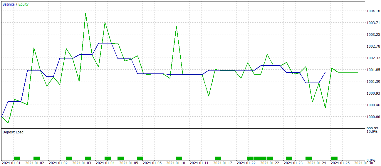
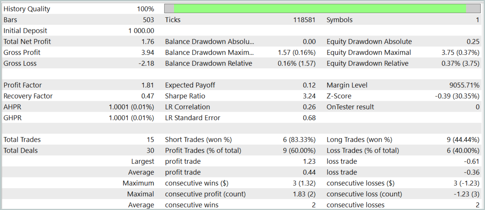
The model achieved a level of 60% profitable trades during the testing phase. Moreover, both the average and maximum profit per position exceeded the corresponding loss metrics.

However, there is a "fly in the ointment". During the test period, the model executed only 15 trades. The balance graph shows that the main profits were obtained at the beginning of the month. And then a flat trend is observed. Therefore, in this case, we can only speak about the potential of the model; to make it viable for longer-term trading, further development is necessary.

Conclusion

The Relative Molecule Attention Transformer (R-MAT) represents a significant advancement in the field of forecasting complex properties. In the context of trading, R-MAT can be seen as a powerful tool for analyzing intricate relationships between various market factors, considering both their relative distances and temporal dependencies.

In the practical part, we implemented our own interpretation of the proposed approaches using MQL5 and trained the resulting models on real-world data. The test results indicate the potential of the proposed solution. However, the model requires further refinement before it can be used in live trading scenarios.

References

Programs used in the article

#	Name	Type	Description
1	Research.mq5	Expert Advisor	EA for collecting examples
2	ResearchRealORL.mq5	Expert Advisor	EA for collecting examples using the Real-ORL method
3	Study.mq5	Expert Advisor	Model training EA
4	Test.mq5	Expert Advisor	Model testing EA
5	Trajectory.mqh	Class library	System state description structure
6	NeuroNet.mqh	Class library	A library of classes for creating a neural network
7	NeuroNet.cl	Library	OpenCL program code library

Translated from Russian by MetaQuotes Ltd.
Original article: https://www.mql5.com/ru/articles/16097

Attached files |

Download ZIP

MQL5.zip (1976.95 KB)

Warning: All rights to these materials are reserved by MetaQuotes Ltd. Copying or reprinting of these materials in whole or in part is prohibited.