Developing a Trading Strategy: The Flower Volatility Index Trend-Following Approach

Introduction

Financial markets move in rhythms—patterns of expansion and contraction, acceleration and slowdown, trend formation and cyclical rotation. Traders have long attempted to model this rhythm mathematically, creating indicators that help define entry opportunities, identify trend direction, or signal when prices have stretched too far from equilibrium. These price-based mathematical models, broadly known as technical indicators, are interpreted in different ways depending on the trader’s objective.

Over the years, several indicators have stood out for mapping cycles and trends or overextended conditions, including the Commodity Channel Index (CCI), Force Index, Bull and Bear Power, Relative Vigor Index (RVI), Cycle Lines, and Fibonacci Time Zones. Each offers a unique lens into market structure.

In this article, we introduce a trend-following strategy derived from a classical mathematical function known as the Rose Curve. Originally studied by Italian mathematician Guido Grandi (1671–1742), the Rose Curve produces geometric flower-like patterns—hence its name. By redefining its parameters, we construct a new oscillator called the Flower Volatility Index (FVI) and then build a trend-trading framework around it.

The Mathematical Foundation: The Rose Curve

The Rose Curve is defined by the polar equation:

Decomposing this radial function yields the Cartesian components:

The function's properties make it exceptionally suitable for building a technical indicator. Its behavior is governed by the rational ratio n/d, which dictates the shape, symmetry, and periodicity of the resulting plot. These components are the foundation upon which we construct the Flower Volatility Index. Before applying this function to market data, it is useful to explore its intrinsic properties.

Figure 1 through 3 below illustrates sample radial plots of the Rose Curve, highlighting its versatility:

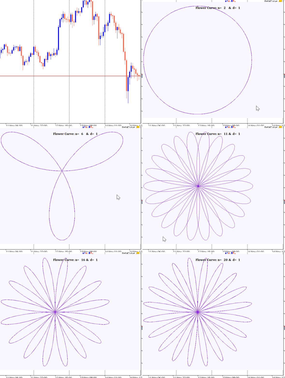
Figure 1: N=20 , d=1

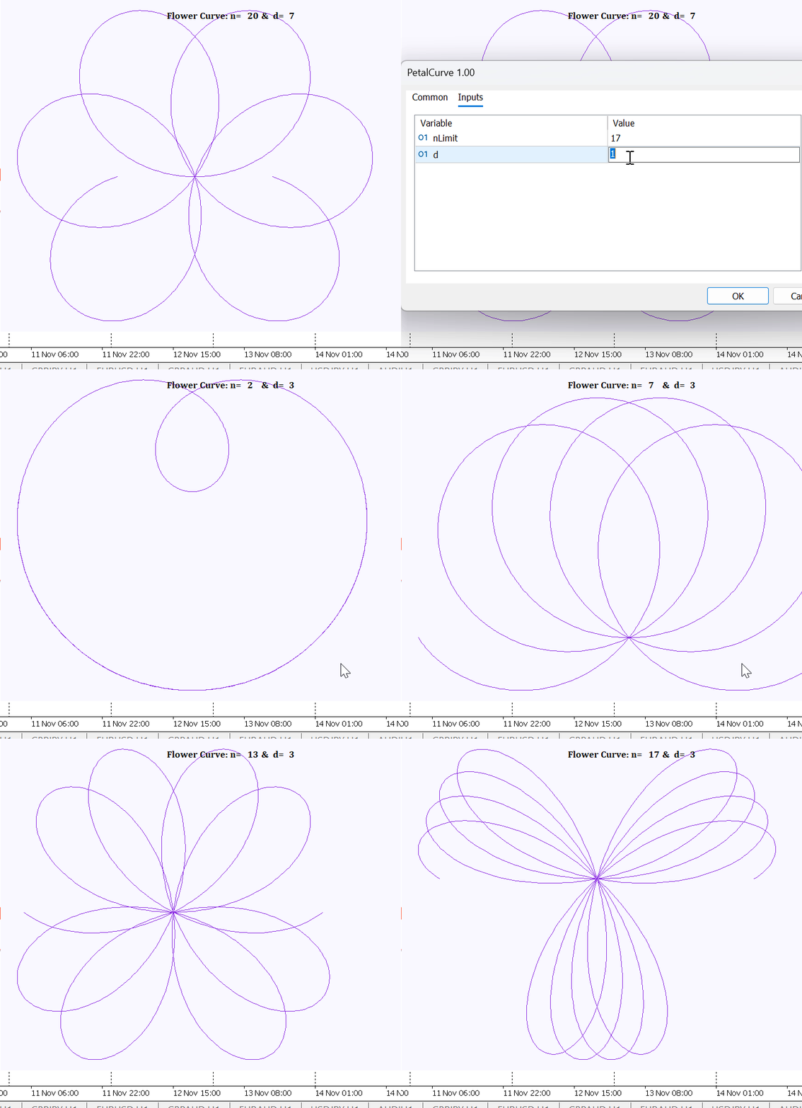
Figure 2: N=17, d=1

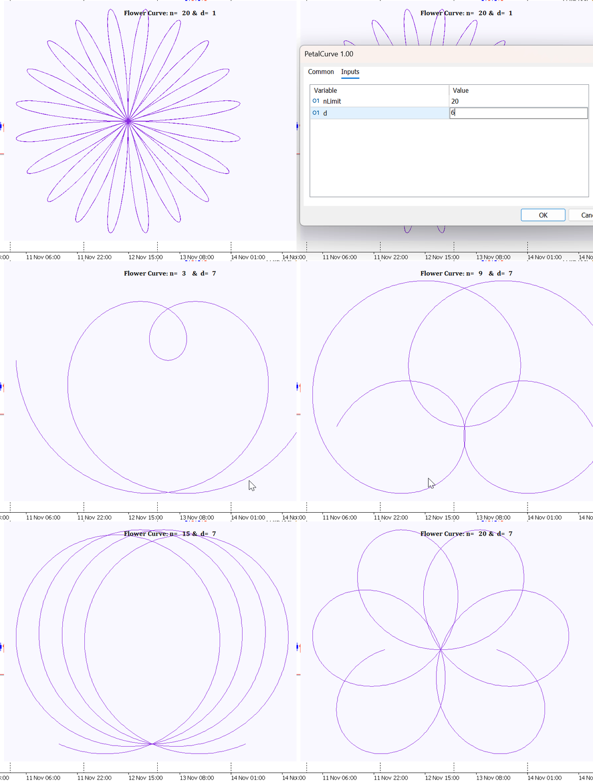
Figure 3: N=20, d=7

Key observations from these radial plots include:

• Pattern Diversity: The ratio n/d generates a wide array of patterns. When rational, it creates symmetric petal-like structures; a ratio of 1/2 produces a simple circle, while higher ratios yield more intricate, multi-lobed designs.

• Petal Count: The key parameter j = n/(2d) determines the number of petals or lobes.

• If j is an integer and odd, the curve has  j  petals. If j is an integer and even, it produces 2j petals. For example; n=6,d=3 then j=1 hence 1 petal.  n = 16 , d = 2 then j=4 hence  8 petals.

• If j is rational but not an integer, more complex and incomplete petal patterns emerge.

• Special case: n =d produces cardioid-like forms

• Symmetry and Oscillation: The curves exhibit consistent rotational and reflection symmetry. Crucially, the amplitude always oscillates between -1 and 1, making it an ideal candidate for a bounded oscillator from which a trader can select components (X or Y) that best suit their strategic needs.

Reviewing the Code Structure for the Rose Curve

To begin constructing the Rose Curve, the first essential step is to include the Canvas library, which provides all necessary properties and functions for rendering graphical objects on the chart. This library serves as the foundation for drawing, plotting, and managing visual elements within the indicator or script.

#include <Canvas\Canvas.mqh>


// Create canvas for drawing
int width = 800;   // Canvas width
int height = 600;  // Canvas height
string canvas_name = "FlowerCurve";

After importing the Canvas library, we define the dimensions of the drawing area. In this example, the canvas width and height are set to 800 and 600 pixels respectively.

The canvas is also assigned an identifiable name, "FlowerCurve", which allows the platform to reference and manage the drawing surface.

Within the CurvePlotting function, the process of generating the Flower (Rose) Curve begins with the creation of the canvas object. This object serves as the drawing surface, and it is configured using the predefined canvas name, its position on the chart, the frame size, and the chosen color format. If the canvas fails to initialize, an error message is printed and the function exits gracefully.

   // Create canvas object
   CCanvas canvas;
   if(!canvas.CreateBitmapLabel(canvas_name, 200, 50, width, height, COLOR_FORMAT_XRGB_NOALPHA))
     {
      Print("Error creating canvas: ", GetLastError());
      return;
     }

   // Set up drawing parameters
   int points = 1000;           // Number of points
   double t_start = -2 * M_PI;           // Start angle
   double t_end = 2 * M_PI;     // End angle
   double step = (t_end - t_start) / (points - 1);
   
   // Calculate curve points
   double x[], y[];
   ArrayResize(x, points);
   ArrayResize(y, points);
   
   for(int i = 0; i < points; i++)
     {
      double t = t_start + i * step;
      double rad = MathSin((n*t)/(2*d));
      y[i] = MathSin(t) * rad;
      x[i] = MathCos(t) * rad;
     }

Once the canvas is successfully created, the function proceeds to set the parameters required for plotting. This includes defining the total number of points to compute, as well as specifying the start and end angles for the curve. A step value is calculated to evenly space the angle increments across the defined interval.

After establishing these parameters, the function initializes arrays to store the x- and y-coordinates of the curve. It then iterates through each point, computing the angle t and evaluating the mathematical expressions that define the Flower Curve.

After computing the raw x and y data points for the Flower Curve, the next task within the CurvePlotting function is to properly scale these coordinates so the entire curve fits neatly within the canvas area. This involves several steps, beginning with identifying the minimum and maximum values for both x and y. These bounds are essential for determining how the curve should be proportionally resized.

   // Find coordinate bounds for scaling
   double x_min = x[ArrayMinimum(x)];
   double x_max = x[ArrayMaximum(x)];
   double y_min = y[ArrayMinimum(y)];
   double y_max = y[ArrayMaximum(y)];
   
   // Scale points to canvas coordinates
   int x_px[], y_px[];
   ArrayResize(x_px, points);
   ArrayResize(y_px, points);
   
   double x_scale = (width - 40) / (x_max - x_min);
   double y_scale = (height - 40) / (y_max - y_min);
   double scale = MathMin(x_scale, y_scale); // Maintain aspect ratio
   
   for(int i = 0; i < points; i++)
     {
      x_px[i] = (int)((x[i] - x_min) * scale) + 30;
      y_px[i] = height - (int)((y[i] - y_min) * scale) - 20; // Flip Y-axis for canvas coordinates
     }

With the extremes identified, the function creates integer arrays ( x_px and y_px ) that will hold the transformed pixel coordinates. Scaling factors for both axes are then calculated based on the available drawing space (leaving margins to avoid touching the edges of the canvas). To preserve the shape of the curve without distortion, the smaller of the two scaling values is selected as the uniform scaling factor.

Finally, each point is converted from mathematical coordinates to canvas coordinates. The x-values are shifted to the right to create a margin, while the y-values are inverted—since canvas coordinates increase downward—ensuring that the plotted curve appears correctly oriented.

The final stage of the CurvePlotting function focuses on rendering the Flower Curve onto the canvas. This begins with setting the background color, ensuring the drawing surface is clean and visually appealing. In this implementation, a GhostWhite background is used to provide a soft contrast against the curve.

Next, the line color is defined. A fully opaque BlueViolet tone is selected, and its ARGB value is passed directly to the canvas’s line-drawing method. The curve itself is plotted as a polyline by drawing consecutive line segments between each pair of scaled data points.

   // Draw the curve
   canvas.Erase(ColorToARGB(clrGhostWhite, 255)); // GhostWhite background

   // Set line color - we'll pass this directly to Line method
    uint line_color = ColorToARGB(clrBlueViolet, 255);
   
   // Draw the polyline
   for(int i = 1; i < points; i++)
     {
      canvas.Line(x_px[i-1], y_px[i-1], x_px[i], y_px[i], line_color);
     }
   
   // Add title
   canvas.FontSet("Cambria", 20, FW_BOLD);
   canvas.TextOut(300, 20, "Flower Curve: n=", ColorToARGB(clrBlack, 255));
   canvas.TextOut(445, 20, IntegerToString(n), ColorToARGB(clrBlack, 255));

   canvas.TextOut(470, 20, "&  d=", ColorToARGB(clrBlack, 255));
   canvas.TextOut(520, 20, IntegerToString(d), ColorToARGB(clrBlack, 255));
   
   // Update display
   canvas.Update();

To complete the visual presentation, the function sets the font style, size, and weight. A Cambria bold font at size 20 is chosen for clarity. The curve title is then rendered at the top of the canvas using canvas.TextOut , dynamically displaying the current values of n and d used in generating the Flower Curve.

Once all elements have been drawn, the canvas.Update() method is called to refresh the display, making all rendered components visible on the chart.

Automating Curve Generation in the Start Function 

In the Start function, the plotting process is automated by placing the CurvePlotting function inside a loop. This structure allows the Flower Curve to be dynamically rendered for different combinations of the input parameters n and d. By adjusting these parameters, the script can display a variety of curve shapes, each reflecting unique mathematical characteristics.

   int p=1;
   while (p<=nLimit) 
    {
    
     CurvePlotting(p);
     p++;
     Sleep(1000);

Both n and d are exposed as user-defined input parameters. This gives the trader or analyst full control over customizing the geometry of the Flower Curve without modifying the core code. When the program runs, it iterates through the designated values, calling  CurvePlotting  for each pair. This enables seamless visualization of multiple curve patterns directly on the chart.

From Geometry to Market Indicator: Constructing the Flower Volatility Index

Before developing the Flower Volatility Index (FVI) oscillator, it is instructive to examine the Cartesian components of the Rose Curve. Translating the polar function into X and Y components reveals its oscillatory nature in a form more familiar to traders.

Figure 4 through 7 displays the X and Y components of the Rose Curve function over time for different values of n and d: The red plot is the X-component and blue plot is the Y-component of the Rose Curve, each plotted against the angle.

Figure 4 : Rose wave: n=5, d=1

Figure 5: Rose wave: n=1, d=1

Figure 6: Rose wave: n=5, d=7

Figure 7:Rose wave: n=20, d=8

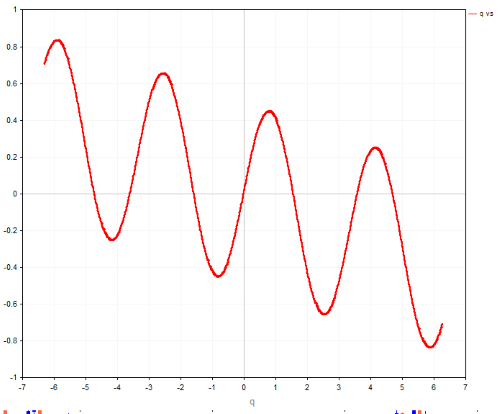
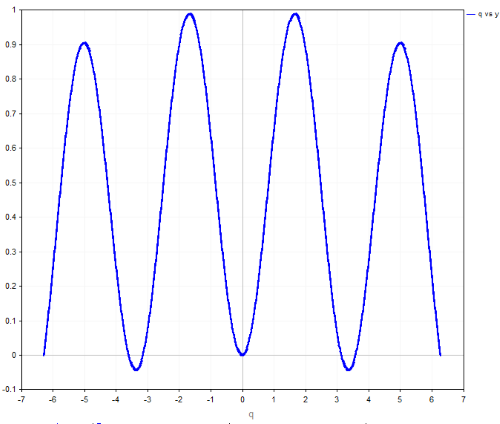
Figure 8:Rose wave: n=7, d=4

Analysis of these Cartesian plots reveals critical characteristics for financial application:

• Bounded Oscillation: Both components consistently oscillate between -1 and 1, providing natural overbought and oversold boundaries.
• Frequency Control: The parameters  n  and  d  offer precise control over the oscillation's frequency. Higher  n  values increase frequency, while higher  d  values decrease it.
• Predictable Periodicity: The period of the oscillation is given by T = 4πd/n. This allows for strategic tuning: a small  n/d  ratio creates longer, smoother cycles ideal for capturing major trends, while a large ratio generates shorter, more reactive cycles.

Special cases further demonstrate its flexibility:

• When  n = d , the function simplifies to  r(q) = sin(q/2) , a basic sine wave.
• When  n = 2d , it becomes  r(q) = sin(q) , a standard sine wave.

Preparing to Plot the Cartesian Coordinates

Before generating the Cartesian form of the curve, the necessary graphical tools must be loaded. This is achieved by including the Graphics library, which provides all the essential functions for plotting, rendering, and managing visual elements within the chart environment. The library serves as the backbone for drawing the x–y components of the Flower Curve.

Once the library is included, a graphic object name is defined. In this case, the plotting surface is identified as "PetalPlot", allowing the program to reference and control the graphical area during rendering.

#include <Graphics/Graphic.mqh>

string g_name = "PetalPlot";

To prepare the chart for plotting the Cartesian components of the Flower Curve, a dedicated function— SetupChartQX —is defined. This function encapsulates all the essential configuration steps needed to create a clean, readable, and visually structured plotting environment. By centralizing these settings, the chart is consistently formatted each time a new curve is rendered.

The function begins by setting a white background, creating a neutral canvas for the graphical elements. It then configures both axes:

• The X-axis spans from −2π to 2π and is labeled q.
• The Y-axis ranges from −1.2 to 1.2 and is labeled x.

void SetupChartQX(CGraphic &graphic)
{
   // Set background color
   graphic.BackgroundColor(clrWhite);
         
   // Configure X axis
   graphic.XAxis().Min(-2*M_PI);
   graphic.XAxis().Max(2*M_PI);
   graphic.XAxis().Name("q");
   
   // Configure Y axis
   graphic.YAxis().Min(-1.2);
   graphic.YAxis().Max(1.2);
   graphic.YAxis().Name("x");
   
   // Add grid
   graphic.XAxis().Color(clrGray);
   graphic.YAxis().Color(clrGray);
   
   // Increase font sizes
   graphic.XAxis().ValuesSize(14);
   graphic.YAxis().ValuesSize(14);
   graphic.XAxis().NameSize(16);
   graphic.YAxis().NameSize(16);
   
   // Add title
   graphic.CurvePlotAll();
   graphic.Update();
}

These ranges ensure that the full variation of the input function can be displayed without clipping.

Gridlines are added by setting the axis colors to gray, improving readability and helping users visually interpret the curve’s position relative to the axes. To enhance clarity further, the font size for axis values and axis names is increased.

Finally, the function calls  CurvePlotAll()  followed by  Update()  to prepare the chart for displaying curve data. 

The PlotQX() function is designed to handle all the plotting operations for the X-component of the Rose Curve. This function serves as the central engine responsible for generating the data points, applying the necessary transformations, and rendering the resulting plot on the chart.

void PlotQX(CGraphic &graphic)
{
   int points = 1000;
   double q[], x[], r[];
   ArrayResize(q, points);
   ArrayResize(x, points);
   ArrayResize(r, points);   
   
   // Generate data points
   for(int i = 0; i < points; i++)
   {
      q[i] = -2*M_PI + (4*M_PI)*i/(points-1);
      r[i] = MathSin(n * q[i] / (2*d));
      x[i] = r[i] * MathCos(q[i]);
   }
  
   // Get the curve object and set line properties
   CCurve* curve = graphic.CurveAdd(q, x, CURVE_LINES, "q vs x");
   if(curve != NULL)
   {
      curve.LinesStyle(STYLE_SOLID);
      curve.LinesWidth(3);
      curve.Color(ColorToARGB(clrRed, 255));
   }   
   graphic.CurvePlotAll();
}

Inside the function, arrays are created to store the computed values of q and x. Using the mathematical formulation of the Flower Curve, the function iterates through a series of evenly spaced q values, computes the corresponding radius term, and derives the X-component.

Plotting the Y-Component: SetupChartQY and PlotQY Functions

Just as the X-component of the Rose Curve is handled through dedicated setup and plotting functions, the Y-component is managed using two parallel functions: SetupChartQY and PlotQY. These functions mirror the structure and purpose of their X-component counterparts, ensuring consistency and clarity across all visual representations.

The SetupChartQY function prepares the chart environment specifically for plotting the Y-component. It configures the background color, axis ranges, axis labels, grid appearance, and font sizes. By doing so, it creates a clean and well-organized visual space tailored for the Y-axis data.

The PlotQY function then handles the computation and rendering of the Y-component. 

The calculated q and y values are plotted onto the prepared chart, with line properties set to give the curve a distinct and readable appearance. After plotting, the function updates the graphic object so the newly drawn curve becomes visible on the chart.

To visualize the Cartesian components of the Rose Curve, separate graphical objects are created for the X-component and Y-component, each with its own plotting window. This ensures that both aspects of the curve can be displayed independently and clearly.

   // Create first graphic object for q vs x
   CGraphic graphic_x;
   
   // Create graphic window for q vs x
   if(!graphic_x.Create(0, g_name + "_q_vs_x", 0, 30, 30, 800, 600))
   {
      Print("Error creating graphic for q vs x!");
      return;
   }

   // Create second graphic object for q vs y
   CGraphic graphic_y;
   
   // Create graphic window for q vs y
   if(!graphic_y.Create(0, g_name + "_q_vs_y", 0, 750, 30, 1500, 600))
   {
      Print("Error creating graphic for q vs y!");
      return;
   }

For the X-component, a graphic object named graphic_x is instantiated. The corresponding graphic window is positioned on the chart with defined coordinates, width, and height, providing a dedicated area for plotting q versus x. If the window creation fails, an error message is printed, and the function exits gracefully.

Similarly, for the Y-component, a second graphic object named graphic_y is created. Its window is positioned separately on the chart, with dimensions set to accommodate the q versus y plot. This separation allows both components to be displayed side by side or in a stacked layout for better visual comparison.

The Indicator: Developing the Flower Volatility Index

With the mathematical foundation of the Rose Curve established, we can now transition from theory to application. The next step is to adapt the Rose Curve into a volatility-sensitive market oscillator—what we call the Flower Volatility Index (FVI).

To achieve this, we replace the traditional angle variable θ in the Rose Curve with a market-derived variable q. This transformation links the geometric properties of the Rose Curve directly to price behavior.

We redefine the angle as q, where: 

Let's break down the components of this critical substitution:

• Close Price - MA (Moving Average): This term represents the price's deviation from its recent mean. A simple or exponential moving average can be used, with the period defining the strategy's sensitivity. This measures the asset's momentum or trend direction. Larger deviations yield larger q  values.
• ATR (Average True Range): Dividing by the ATR standardizes the deviation, creating a unitless measure. This crucial step accounts for market volatility, ensuring the indicator adapts to changing market conditions. A large price move in a low-volatility environment will have a more significant impact than the same move in a high-volatility environment.
• Scalar k: This is a tuning coefficient that allows the trader to control the sensitivity of the  q  oscillator. A higher  k  value amplifies the deviations, making the FVI more reactive.

By substituting q into the Rose Curve, the indicator becomes sensitive to both trend displacement and volatility conditions, producing smoother and more interpretable oscillatory signals.

Full Indicator Formula

By substituting the market-derived q into the Rose Curve definitions, the complete Flower Volatility Index becomes:

X-Component FVI:

Y-Component FVI:

Although both oscillators remain bounded within the range [−1,+1], producing normalized and stable signals across all market conditions, an important nuance emerges when examining different parameter combinations of  n and d. As illustrated in Figures 4 to 8, certain configurations cause either the x-component or y-component of the Flower Volatility Index to become asymmetrical. In these cases, the oscillator may spend more time in positive territory than negative (or vice versa), creating a structural bias within the waveform.

This asymmetry stems from the geometric properties of the Rose Curve and becomes more pronounced when n/d produces incomplete petals or uneven rotational symmetry. When such parameter combinations are paired with the market-derived variable q, the resulting oscillator can become directionally biased—favoring one side of the zero line for extended periods.

Rather than being a flaw, this characteristic offers a powerful opportunity: a naturally biased oscillator can help identify dominant long-term trends or persistent one-directional market phases. For this reason, the indicator allows the user to select either the X-component or the Y-component, enabling traders to intentionally exploit this asymmetry depending on their strategy objective. 

FVI Indicator Demonstration

At this point, let us examine how the Flower Volatility Index behaves in practice.

The FVI is highly responsive to its input parameters, and modifying any of these values—whether the MA period, ATR period, sensitivity constant k, or the choice between X- and Y-components—directly influences the shape and responsiveness of the oscillator. This flexibility allows traders to tailor the indicator to “sync” with the rhythm of the specific market or instrument they are trading.

The true strategic advantage of the FVI lies in its tunable complexity. By carefully adjusting the Rose Curve parameters n, d, and the scaling parameter k, the trader can design an oscillator that behaves in remarkably different ways:

• Trend Identification: Sustained values of FVI above zero can be interpreted as bullish momentum, while values below zero suggest bearish momentum.

• Signal Generation: The crossing of the FVI line above or below its zero centerline, or the oscillation between its extremes, can generate buy and sell signals for a trend-following system.

• Volatility-Adaptive: The incorporation of ATR makes the FVI a dynamic indicator. In high-volatility periods, it becomes less sensitive, preventing whipsaws. In low-volatility periods, it becomes more sensitive, allowing for earlier entry into new trends.

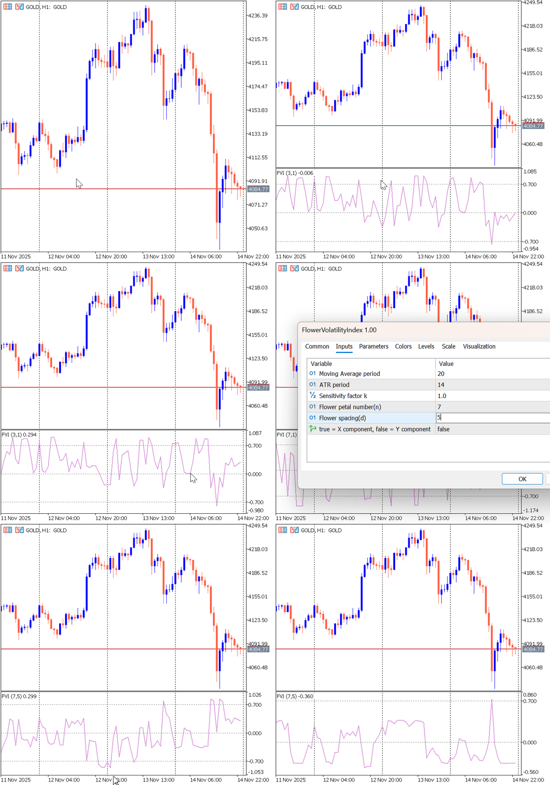
Figure 9: FVI Indicator 

Throughout these changes, the FVI remains entirely volatility-normalized through its dependence on ATR. This ensures that the oscillator adapts automatically to changing market regimes—expanding in quiet markets and compressing in volatile ones—while maintaining consistent interpretability across asset classes and time frames.

The Expert Advisor: FVI Trend Following Strategy

This Expert Advisor uses the FVI for signal generation and the Awesome Oscillator (AO) as the trend filter. Trades are executed only when volatility-driven momentum (FVI) aligns with the prevailing trend (AO).

The EA's decision-making process is governed by the following concrete rules:

1. Sell Condition: 

A sell trade is opened when:

• AO < 0 (downtrend), and
• FVI crosses above +0.7 (strong upward exhaustion within a bearish trend)

2. Buy Condition:

A buy trade is opened when:

• AO > 0 (uptrend), and
• FVI crosses below −0.7 (strong downward exhaustion within a bullish trend)

3. Exit Condition:

• Trades close using Take Profit and Stop Loss levels.

4. Multiple Entry Rule:

• Single Position Per Side: The EA will open only one position for a given trade direction. For example, if a buy position is already open, it will not open another buy position until the first is closed. However, it can open a sell position if its conditions are met, allowing the strategy to capture trend reversals.
• Entry Cooldown Period: To prevent excessive trading and "echo" signals, the EA will implement a cooldown period. After an entry signal is executed, the EA will wait for a specified number of bars (e.g., 10 bars) before checking for and acting upon a new entry signal for either direction. This manages trade frequency and ensures signals have time to develop.

Understanding the Code Structure of the FVI Expert Advisor

At the core of the FV Expert Advisor (EA) is the CalculateFVI() function, which is responsible for computing the FVI values used in the trading logic. This function processes key input parameters—namely the MA, ATR, and the curve parameters n, d, and k—to generate the indicator output.

void CalculateFVI()
{
    prevFVI = curFVI;

    // Get indicator values
    double ma[1], atr[1], ao[1];
    double close = iClose(_Symbol, _Period, 1);
    
    // Copy indicator values
    if(CopyBuffer(maHandle, 0, 1, 1, ma) < 1 || 
       CopyBuffer(atrHandle, 0, 1, 1, atr) < 1)
    {
        Print("Error copying indicator buffers");
        return;
    }

    // Calculate q
    double q = k * (close - ma[0]) / (atr[0] > 0 ? atr[0] : 1);

    // Calculate r(q)
    double r = MathSin(n * q / (2 * d));

    // Calculate FVI based on selected component
    if(Use_X_Component)
        curFVI = r * MathCos(q); // X component
    else
        curFVI = r * MathSin(q); // Y component
}

The computation begins by storing the previous FVI value, allowing the EA to compare past and current values when evaluating trade conditions. It then retrieves the most recent closing price and copies the MA and ATR values from their respective indicator buffers. Proper error handling ensures the EA gracefully exits if indicator data cannot be accessed.

The CheckForEntry() function serves as the decision-making engine of the FVI EA. Its primary role is to ensure that all entry conditions are satisfied before any trade is executed, thereby maintaining discipline and preventing premature or invalid order placement.

The function begins by verifying that a sufficient number of bars have passed since the last trade. This spacing mechanism helps avoid rapid consecutive entries, especially during volatile market conditions. Once the minimum bar requirement is met, the function evaluates the predefined FVI-based entry rules—whether the current and previous FVI values satisfy the criteria for a bullish or bearish setup.

void CheckForEntry()
{
    // Check minimum bars between entries
    if(barsSinceLastTrade < MinBarsBtwEntries)
        return;

    // Get Awesome Oscillator value
    double ao[1];
    if(CopyBuffer(aoHandle, 0, 1, 1, ao) < 1)
    {
        Print("Error copying AO buffer");
        return;
    }

    // Check for buy conditions
    if(ao[0] > 0 && prevFVI > -0.7 && curFVI < -0.7)
    {
        if(CountPositions(POSITION_TYPE_BUY) == 0)
        {
            OpenBuyOrder();
            barsSinceLastTrade = 0;
        }
    }

    // Check for sell conditions
    if(ao[0] < 0 && prevFVI < 0.7 && curFVI > 0.7)
    {
        if(CountPositions(POSITION_TYPE_SELL) == 0)
        {
            OpenSellOrder();
            barsSinceLastTrade = 0;
        }
    }
}

If a valid buy signal is detected, the EA triggers the OpenBuyOrder() function to submit a buy order to the broker’s terminal. Similarly, if a sell signal is confirmed, the OpenSellOrder() function is executed to open a sell position.

After a trade is successfully placed, the counter barsSinceLastTrade is reset to zero, ensuring that the EA once again respects the required spacing before initiating the next trade.

Through this structure, the CheckForEntry() function provides a reliable and efficient framework for managing trade execution, ensuring that positions are opened only under well-defined and controlled conditions.

FVI EA Demonstration

The Expert Advisor includes a comprehensive set of input parameters—covering both trading settings and  FVI parameters—that allow traders to fine-tune performance. These inputs are fully accessible for optimization, enabling users to adjust variables such as risk settings, sensitivity parameters and FVI computation values. As illustrated in Figure 10, the optimization interface provides a structured way to experiment with different parameter combinations, helping traders identify the most effective configuration for various market conditions.

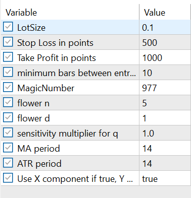
Figure 10: EA input values

Figure 11 illustrates how the Expert Advisor executes trades based on the defined trading logic. Once the market conditions align with the specified entry rules, the EA automatically triggers buy or sell positions, managing each execution according to the configured risk parameters and FVI-based signals. This visual representation helps demonstrate the flow from signal generation to order placement, showcasing the EA’s ability to respond systematically to market movements.

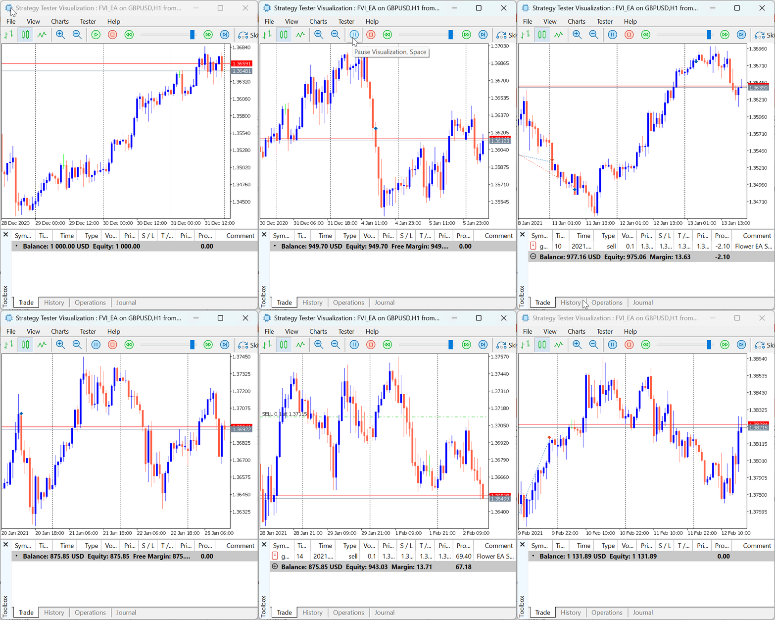
Figure 11: FVI EA Demonstration

Conclusion

This article has introduced the Flower Volatility Index (FVI), a novel approach that transforms the mathematical elegance of Rose Curves into a functional trading tool. By mapping market volatility and price displacement through the Flower Curve’s X- and Y-components, we demonstrated how the FVI can be used to detect directional bias, trend strength, and potential turning points.

The article also outlined the complete structure of the FVI Expert Advisor — from curve plotting and graphical rendering to signal generation and automated trade execution. Through this work, we have shown how mathematical models can be adapted into practical trading mechanisms capable of supporting both analysis and decision-making in real market conditions.

Overall, the study highlights the potential of geometric and trigonometric functions as alternative frameworks for understanding market behaviour.

In our next work, we will test the strategy standalone and with other indicators to find its suitable pairs under various financial instruments. Until then, happy trading.

Files	Description
PetalCurve.mq5	This script file plots the Rose Curves. The chart can be removed when the template is updated or replaced.
PetalWaves.mq5	The script file plots the X & Y component of the Curves showing as wave pattern. Update the template to remove the plotted charts.
FlowerVolatilityIndex.mq5	This indicator file plots the Flower Volatility Index in a separate window.
FVI_EA.mq5	This file contains the EA the executes trades automatically.