Neural Networks in Trading: Hierarchical Dual-Tower Transformer (Hidformer)

Introduction

Neural network models capable of capturing the temporal structure of data and identifying hidden patterns have become particularly in demand in financial forecasting. However, traditional neural network approaches face limitations related to high computational complexity and insufficient interpretability of results. Consequently, in recent years, architectures based on attention mechanisms have attracted increasing interest from researchers, as they provide more accurate analysis of time series and financial data.

Models based on the Transformer architecture and its modifications have gained the most popularity. One such modification, introduced in the paper "Hidformer: Transformer-Style Neural Network in Stock Price Forecasting" is called Hidformer. This model is specifically designed for time-series analysis and focuses on improving prediction accuracy through optimized attention mechanisms, efficient identification of long-term dependencies, and adaptation to the characteristics of financial data. The main advantage of Hidformer lies in its ability to account for complex temporal relationships, which is an especially important feature in stock market analysis, where asset prices depend on numerous factors.

The authors of the framework propose improved processing of temporal dependencies, reduced computational complexity, and enhanced prediction accuracy. This makes Hidformer a promising tool for financial analysis and forecasting.

Hidformer Algorithm

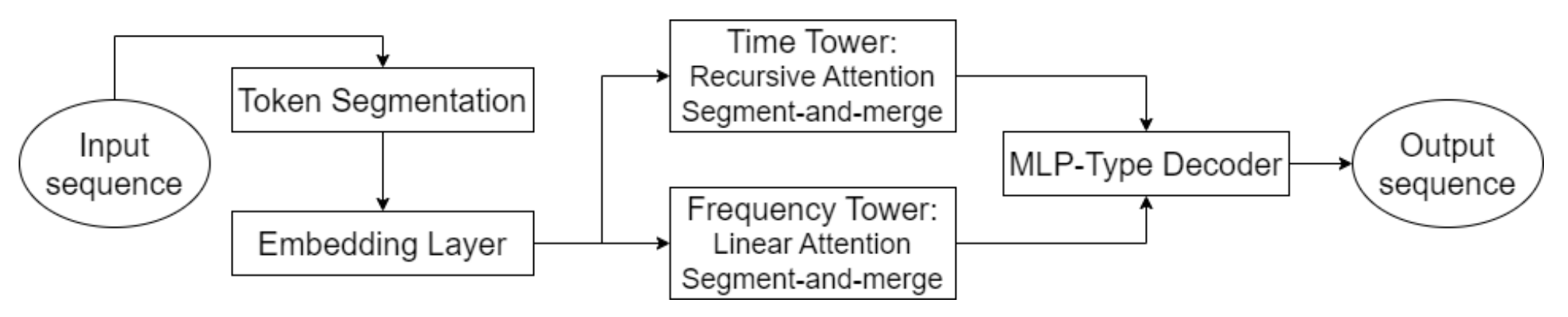
One of the key features of Hidformer is the parallel processing of data by two encoders. The first analyzes temporal characteristics, identifying trends and patterns over time. The second operates in the frequency domain, which allows the model to identify deeper dependencies and eliminate market noise. This approach helps reveal hidden patterns in data. This is critical in forecasting stock prices, where signals can be masked by noise. The input data is split into subsequences, which are then merged at each processing stage, improving the detection of significant patterns.

This method is particularly useful for analyzing volatile assets such as technology stocks or cryptocurrencies, as it helps separate fundamental trends from short-term fluctuations. Instead of the standard multi-head attention used in the Transformer architecture, the authors of Hidformer propose using a recursive attention mechanism in the temporal encoder and a linear attention mechanism to identify dependencies in the frequency spectrum. This reduces computational resource consumption and improves prediction stability, making the model efficient when working with large volumes of market data.

The model's decoder is based on a multilayer perceptron, allowing it to forecast the entire sequence of prices in a single step. As a result, errors that would otherwise accumulate during step-by-step forecasting are eliminated. This architecture is especially advantageous for financial forecasting because it reduces the likelihood of accumulating inaccuracies in long-term predictions.

The original visualization of the Hidformer framework is provided below.

Implementation in MQL5

After briefly reviewing the theoretical aspects of the Hidformer framework, we now move on to implementing our own interpretation of the proposed approaches using MQL5. We will begin by implementing the modified attention algorithms.

First, let's look at the recursive attention algorithm. Initially proposed for solving visual dialog problems, the recursive attention mechanism helps determine the correct context of the current query based on the preceding dialog history. Clearly, recursive processing of data, compared to parallel computation of multi-head attention, only complicates our task. On the other hand, the recursive approach allows us to avoid processing the entire history by stopping at the nearest relevant element containing the required context.

Such considerations lead us to the construction of a multi-scale attention algorithm. Previously, we discussed various approaches for capturing local and global features by adjusting the attention window. But earlier, different attention levels were used in separate components. Now, I propose modifying the earlier multi-head attention algorithm so that each head receives its own context window. Moreover, we propose defining the context window not around the analyzed element, but starting from the beginning of the sequence. The newest data is stored at the beginning of the sequence. This approach allows us to evaluate the analyzed history in the context of the current market situation.

Attention Modification in OpenCL

To start, we will implement the changes described above on the OpenCL side. For this purpose, we will create a new kernel MultiScaleRelativeAttentionOut, copying most of its code from the donor kernel MHRelativeAttentionOut. The kernel's parameter list is transferred unchanged.

__kernel void MultiScaleRelativeAttentionOut(__global const float * q,        ///<[in] Matrix of Querys
                                             __global const float * k,        ///<[in] Matrix of Keys
                                             __global const float * v,        ///<[in] Matrix of Values
                                             __global const float * bk,       ///<[in] Matrix of Positional Bias Keys
                                             __global const float * bv,       ///<[in] Matrix of Positional Bias Values
                                             __global const float * gc,       ///<[in] Global content bias vector
                                             __global const float * gp,       ///<[in] Global positional bias vector
                                             __global float * score,          ///<[out] Matrix of Scores
                                             __global float * out,            ///<[out] Matrix of attention
                                             const int dimension              ///< Dimension of Key
                                            )
  {
//--- init
   const uint q_id = get_global_id(0);
   const uint k_id = get_local_id(1);
   const uint h = get_global_id(2);
   const uint qunits = get_global_size(0);
   const uint kunits = get_local_size(1);
   const uint heads = get_global_size(2);
   const int shift_q = dimension * (q_id * heads + h);
   const int shift_kv = dimension * (heads * k_id + h);
   const int shift_gc = dimension * h;
   const int shift_s = kunits * (q_id *  heads + h) + k_id;
   const int shift_pb = q_id * kunits + k_id;
   const uint ls = min((uint)get_local_size(1), (uint)LOCAL_ARRAY_SIZE);
   const uint window = fmax((kunits + h) / (h + 1), fmin(3, kunits));
   float koef = sqrt((float)dimension);

Inside the method, we first implement preparatory work. Here we define all the necessary constants, including the context window.

Note that we did not create a separate buffer for passing individual context sizes for each attention head. Instead, we simply divided the length of the analyzed sequence by the attention head ID plus one (since IDs start at zero). Thus, the first head analyzes the entire sequence, and subsequent heads operate on progressively smaller context windows.

Next, we determine the attention coefficients. Each execution thread computes one coefficient for a specific element. However, operations are performed only within the context window. Elements outside the window automatically receive zero attention weight.

   __local float temp[LOCAL_ARRAY_SIZE];
//--- score
   float sc = 0;
   if(k_id < window)
     {
      for(int d = 0; d < dimension; d++)
        {
         float val_q = q[shift_q + d];
         float val_k = k[shift_kv + d];
         float val_bk = bk[shift_kv + d];
         sc += val_q * val_k + val_q * val_bk + val_k * val_bk + gc[shift_q + d] * val_k + 
                                                                 gp[shift_q + d] * val_bk;
        }
      sc = sc / koef;
     }

To improve coefficient stability, we shift the values into the numerical stability region. To do this, we find the maximum coefficient among the calculated values, excluding elements outside the context window.

//--- max value
   for(int cur_k = 0; cur_k < kunits; cur_k += ls)
     {
      if(k_id < window)
         if(k_id >= cur_k && k_id < (cur_k + ls))
           {
            int shift_local = k_id % ls;
            temp[shift_local] = (cur_k == 0 ? sc : fmax(temp[shift_local], sc));
           }
      barrier(CLK_LOCAL_MEM_FENCE);
     }
   uint count = min(ls, kunits);
//---
   do
     {
      count = (count + 1) / 2;
      if(k_id < (window + 1) / 2)
         if(k_id < ls)
            temp[k_id] = (k_id < count && (k_id + count) < kunits ? fmax(temp[k_id + count],
                                                                  temp[k_id]) : temp[k_id]);
      barrier(CLK_LOCAL_MEM_FENCE);
     }
   while(count > 1);

Only then do we compute the exponential of each coefficient minus the maximum value.

   if(k_id < window)
      sc = IsNaNOrInf(exp(fmax(sc - temp[0], -120)), 0);
   barrier(CLK_LOCAL_MEM_FENCE);

However, special attention must be paid to operations within the context window. By shifting the maximum to zero, we make the maximum exponent equal to one. All other coefficients fall between 0 and 1. This improves the stability of the SoftMax function. But since coefficients outside the context window were automatically set to zero, computing their exponent would yield the maximum weight, which is highly undesirable. Therefore, we must preserve their value as zero.

We then sum the coefficients within the workgroup.

//--- sum of exp
   for(int cur_k = 0; cur_k < kunits; cur_k += ls)
     {
      if(k_id >= cur_k && k_id < (cur_k + ls))
        {
         int shift_local = k_id % ls;
         temp[shift_local] = (cur_k == 0 ? 0 : temp[shift_local]) + sc;
        }
      barrier(CLK_LOCAL_MEM_FENCE);
     }
//---
   count = min(ls, (uint)kunits);
   do
     {
      count = (count + 1) / 2;
      if(k_id < count && k_id < (window + 1) / 2)
         temp[k_id] += ((k_id + count) < kunits ? temp[k_id + count] : 0);
      if(k_id + count < ls)
         temp[k_id + count] = 0;
      barrier(CLK_LOCAL_MEM_FENCE);
     }
   while(count > 1);

Next, we normalize each coefficient by dividing it by the computed sum.

//--- score
   float sum = IsNaNOrInf(temp[0], 1);
   if(sum <= 1.2e-7f)
      sum = 1;
   sc /= sum;
   score[shift_s] = sc;
   barrier(CLK_LOCAL_MEM_FENCE);

The normalized coefficients are then written to the corresponding data buffer.

After obtaining normalized attention weights for sequence elements, we can compute the adjusted value of the current element. To do this, we iterate through the sequence, multiply the Value tensor by each coefficient, and sum the results.

//--- out
   int shift_local = k_id % ls;
   for(int d = 0; d < dimension; d++)
     {
      float val_v = v[shift_kv + d];
      float val_bv = bv[shift_kv + d];
      float val = IsNaNOrInf(sc * (val_v + val_bv), 0);
      //--- sum of value
      for(int cur_v = 0; cur_v < kunits; cur_v += ls)
        {
         if(k_id >= cur_v && k_id < (cur_v + ls))
            temp[shift_local] = (cur_v == 0 ? 0 : temp[shift_local]) + val;
         barrier(CLK_LOCAL_MEM_FENCE);
        }
      //---
      count = min(ls, (uint)kunits);
      do
        {
         count = (count + 1) / 2;
         if(k_id < count && (k_id + count) < kunits)
            temp[k_id] += temp[k_id + count];
         if(k_id + count < ls)
            temp[k_id + count] = 0;
         barrier(CLK_LOCAL_MEM_FENCE);
        }
      while(count > 1);
      //---
      if(k_id == 0)
         out[shift_q + d] = IsNaNOrInf(temp[0], 0);
      barrier(CLK_LOCAL_MEM_FENCE);
     }
  }

The outputs are stored in the designated data buffer.

Preserved zero weights allow us to use existing tools for implementing backpropagation algorithms. This completes our work on the OpenCL side. The full source code is provided in the attachment.

Creating Multi-Scale Attention Objects

Next, we need to create multi-scale attention objects in the main program. To maximize the benefits of object inheritance, we simply created Self-Attention and Cross-Attention objects based on existing methods, overriding only the method that calls the newly created kernel. The structure of the new objects is shown below.

class CNeuronMultiScaleRelativeSelfAttention   :  public CNeuronRelativeSelfAttention
  {
protected:
   //---
   virtual bool      AttentionOut(void);

public:
                     CNeuronMultiScaleRelativeSelfAttention(void) {};
                    ~CNeuronMultiScaleRelativeSelfAttention(void) {};
   //---
   virtual int       Type(void) override   const   {  return defNeuronMultiScaleRelativeSelfAttention; }
  };

class CNeuronMultiScaleRelativeCrossAttention   :  public CNeuronRelativeCrossAttention
  {
protected:
   virtual bool      AttentionOut(void);

public:
                     CNeuronMultiScaleRelativeCrossAttention(void) {};
                    ~CNeuronMultiScaleRelativeCrossAttention(void) {};
   //---
   virtual int       Type(void) override   const   {  return defNeuronMultiScaleRelativeCrossAttention; }
  };

We used the classic method of queuing the kernel for execution. We have already reviewed similar methods many times. I believe you will have no difficulty understanding them. Full code for these methods is provided in the appendix.

Recursive Attention Object

The multi-scale attention objects implemented above enable us to analyze data at various context window sizes, but this is not the recursive attention mechanism proposed by the Hidformer authors. We have merely completed the preparatory stage.

Our next step is to build a recursive attention object capable of analyzing current data in the context of previously observed history. For this, we will use some memory module design techniques. Specifically, we will store the context of observed states for a defined historical depth, which will then be used to assess the current state. We will implement this algorithm within the CNeuronRecursiveAttention method, whose structure is shown below.

class CNeuronRecursiveAttention  :  public CNeuronMultiScaleRelativeCrossAttention
  {
protected:
   CNeuronMultiScaleRelativeSelfAttention cSelfAttention;
   CNeuronTransposeOCL  cTransposeSA;
   CNeuronConvOCL       cConvolution;
   CNeuronEmbeddingOCL  cHistory;
   //---
   virtual bool      feedForward(CNeuronBaseOCL *NeuronOCL) override;
   virtual bool      feedForward(CNeuronBaseOCL *NeuronOCL, CBufferFloat *SecondInput)
   override  { return false; }
   virtual bool      calcInputGradients(CNeuronBaseOCL *NeuronOCL) override;
   virtual bool      calcInputGradients(CNeuronBaseOCL *NeuronOCL, CBufferFloat *SecondInput,
                                        CBufferFloat *SecondGradient,
                                        ENUM_ACTIVATION SecondActivation = None)
   override  { return false; }
   virtual bool      updateInputWeights(CNeuronBaseOCL *NeuronOCL) override;
   virtual bool      updateInputWeights(CNeuronBaseOCL *NeuronOCL, CBufferFloat *SecondInput)
   override  { return false; }

public:
                     CNeuronRecursiveAttention(void) {};
                    ~CNeuronRecursiveAttention(void) {};
   //---
   virtual bool      Init(uint numOutputs, uint myIndex, COpenCLMy *open_cl,
                          uint window, uint window_key, uint units_count,
                          uint heads, uint history_size,
                          ENUM_OPTIMIZATION optimization_type, uint batch);
   //---
   virtual int       Type(void) override   const   {  return defNeuronRecursiveAttention; }
   //---
   virtual bool      Save(int const file_handle) override;
   virtual bool      Load(int const file_handle) override;
   //---
   virtual bool      WeightsUpdate(CNeuronBaseOCL *source, float tau) override;
   virtual void      SetOpenCL(COpenCLMy *obj) override;
   //---
   virtual bool      Clear(void) override;
  };

The parent class in this case is the previously implemented multi-scale cross-attention object.

Inside the method, we see a familiar set of overridden virtual methods and several internal objects whose functions we will explore during the implementation of feed-forward and backpropagation passes.

All internal objects are declared static, allowing us to leave the class constructor and destructor empty. Initialization of all inherited and newly declared objects occurs in the Init method.

bool CNeuronRecursiveAttention::Init(uint numOutputs, uint myIndex, COpenCLMy *open_cl,
                                        uint window, uint window_key, uint units_count,
                                                         uint heads, uint history_size,
                                       ENUM_OPTIMIZATION optimization_type, uint batch)
  {
   if(!CNeuronMultiScaleRelativeCrossAttention::Init(numOutputs, myIndex, open_cl, window,
                                               window_key, units_count, heads, window_key,
                                                  history_size, optimization_type, batch))
      return false;

The method parameters include a number of constants that clearly define the architecture of the created object. It is important to note that, despite inheriting from the cross-attention class, our object operates with a single stream of input data. The second data stream required for the correct functioning of the parent class is generated internally. The sequence length of this second stream is defined by the historical depth parameter history_size.

As usual, we immediately call the parent class method of the same name, passing it the necessary parameters. Recall that the parent method already includes all required control points and initialization procedures for inherited objects, including base interfaces.

Next, we initialize the newly declared internal objects. The first is the multi-scale Self-Attention module.

   int index = 0;
   if(!cSelfAttention.Init(0, index, OpenCL, iWindow, iWindowKey, iUnits, iHeads, 
                                                           optimization, iBatch))
      return false;

Using this object allows us to determine which elements of the original data exert the greatest influence on the current state of the analyzed financial instrument.

We then need to add the context of the current environment state to the memory of our recursive attention block. We want to preserve the context of individual univariate sequences. Therefore, we first transpose the input data.

   index++;
   if(!cTransposeSA.Init(0, index, OpenCL, iUnits, iWindow, optimization, iBatch))
      return false;

Then we extract the context of unitary sequences using a convolutional layer.

   index++;
   if(!cConvolution.Init(0, index, OpenCL, iUnits, iUnits, iWindowKey, 1, iWindow,
                                                            optimization, iBatch))
      return false;

Note that the convolutional layer parameters specify a single element of the analyzed sequence, while the number of unitary sequences is passed as the number of independent variables. This allows for completely independent analysis of unitary sequences, as each uses its own set of trainable parameters. This enables deeper analysis of the original multimodal sequence.

Next, we use an embedding generation layer to capture the context of the analyzed environment state and add it to the historical memory stack.

   index++;
   uint windows[] = { iWindowKey * iWindow };
   if(!cHistory.Init(0, index, OpenCL, iUnitsKV, iWindowKey, windows))
      return false;
//---
   return true;
  }

After all operations are successfully completed, we return a logical success value to the calling program and finish the method.

Our next step is to implement the feedForward method, whose algorithm is fairly linear.

bool CNeuronRecursiveAttention::feedForward(CNeuronBaseOCL *NeuronOCL)
  {
   if(!cSelfAttention.FeedForward(NeuronOCL))
      return false;

The method receives a pointer to the input data object containing the multimodal time series. We immediately pass this pointer to the Self-Attention module to analyze dependencies in the current environmental state. The results are then transposed for further processing.

   if(!cTransposeSA.FeedForward(cSelfAttention.AsObject()))
      return false;

We extract the context of unitary sequences using the convolutional layer.

   if(!cConvolution.FeedForward(cTransposeSA.AsObject()))
      return false;

We pass the prepared data to the embedding generator, which extracts the context of the analyzed state and adds it to the memory stack.

   if(!cHistory.FeedForward(cConvolution.AsObject()))
      return false;

Now we need to enrich the previously obtained Self-Attention results with the context of the historical sequence. For this purpose, we use the corresponding method of the parent class, passing it the necessary information.

   return CNeuronMultiScaleRelativeCrossAttention::feedForward(cSelfAttention.AsObject(),
                                                                   cHistory.getOutput());
  }

It is worth noting that, to analyze the current state in the context of previously observed states, we use the multi-scale attention object created earlier. This approach assigns greater weight to recently observed data while reducing the influence of older information. Nevertheless, we still retain the ability to extract key points from the "depths of memory".

Before concluding the method, we return a boolean value indicating the success or failure of the initialization to the caller.

Because the Self-Attention results are used twice in the feed-forward pass, this affects the backpropagation algorithm implemented in the calcInputGradients method.

bool CNeuronRecursiveAttention::calcInputGradients(CNeuronBaseOCL *NeuronOCL)
  {
   if(!NeuronOCL)
      return false;

The backpropagation method receives a pointer to the same input data object, but now we must pass to it the gradient of the error corresponding to its influence on the model's output.

Inside the method, we immediately verify the validity of the received pointer. Otherwise, we cannot pass data to a non-existent object, and further operations lose meaning. Therefore, we continue only if this control point is successfully passed.

As you know, the information flow of the feed-forward and backpropagation passes fully corresponds conceptually, differing only in direction. The feed-forward pass ends with a call to the parent class method. Accordingly, the backpropagation pass begins with a call to its inherited method. The latter distributes the previously received gradient between the two data streams based on their contribution to the final result.

   if(!CNeuronMultiScaleRelativeCrossAttention::calcInputGradients(cSelfAttention.AsObject(),
                                                                        cHistory.getOutput(),
                                                                      cHistory.getGradient(),
                                                     (ENUM_ACTIVATION)cHistory.Activation()))
      return false;

We first distribute the gradient through the auxiliary data stream corresponding to the object's memory. Here, we propagate the error down to the convolutional layer that extracts the context of univariate sequences.

   if(!cConvolution.calcHiddenGradients(cHistory.AsObject()))
      return false;

Then we propagate it further to the transposition layer of the Self-Attention block.

   if(!cTransposeSA.calcHiddenGradients(cConvolution.AsObject()))
      return false;

Next, we must pass the gradient down to the multi-scale Self-Attention layer. But earlier, we already propagated to it the gradient of the main data stream, which must be preserved. For this, we temporarily swap the pointers to the data buffers. First we pass to the object a pointer to a free buffer while saving the existing one.

   CBufferFloat *temp = cSelfAttention.getGradient();
   if(!cSelfAttention.SetGradient(cTransposeSA.getPrevOutput(), false) ||
      !cSelfAttention.calcHiddenGradients(cTransposeSA.AsObject()) ||
      !SumAndNormilize(temp, cSelfAttention.getGradient(), temp, iWindow, false, 0, 0, 0, 1) ||
      !cSelfAttention.SetGradient(temp, false))
      return false;

We then propagate the error gradient and sum the values from both data streams. After that, we restore the buffer pointers to their original state.

Finally, we propagate the gradient to the level of the input data.

   if(!NeuronOCL.calcHiddenGradients(cSelfAttention.AsObject()))
      return false;
//---
   return true;
  }

At the end of the method, we return a logical success value.

The full code of this object and all its methods is provided in the attachment for further study.

Linear Attention Object

In addition to the implemented recursive attention object, the authors of the framework also proposed using linear attention in the tower responsible for frequency spectrum analysis.

Linear Attention is one of the approaches for optimizing the traditional attention mechanism in transformers. Unlike classical Self-Attention, which relies on fully connected matrix operations with quadratic complexity, linear attention reduces computational complexity, making it efficient for processing long sequences.

Linear attention introduces factorizations φ(Q) and φ(K), allowing the attention computation to be represented as:

Advantages of Linear Attention

1. Linear complexity: Reduced computation costs, making it possible to process long sequences.
2. Lower memory consumption: No need to store the full Score matrix of dependency coefficients, reducing memory requirements.
3. Efficiency in online tasks: Linear attention supports streaming data processing since updates occur incrementally.
4. Flexibility in kernel selection: Different φ(x) functions allow the attention mechanism to be adapted to specific tasks.

The implementation of the linear attention algorithm is encapsulated in the CNeuronLinerAttention object, whose structure is presented below.

class CNeuronLinerAttention   :  public CNeuronBaseOCL
  {
protected:
   uint                 iWindow;
   uint                 iWindowKey;
   uint                 iUnits;
   uint                 iVariables;
   //---
   CNeuronConvOCL       cQuery;
   CNeuronConvOCL       cKey;
   CNeuronTransposeVRCOCL  cKeyT;
   CNeuronBaseOCL       cKeyValue;
   CNeuronBaseOCL       cAttentionOut;
   //---
   virtual bool      feedForward(CNeuronBaseOCL *NeuronOCL) override;
   virtual bool      calcInputGradients(CNeuronBaseOCL *NeuronOCL) override;
   virtual bool      updateInputWeights(CNeuronBaseOCL *NeuronOCL) override;

public:
                     CNeuronLinerAttention(void) {};
                    ~CNeuronLinerAttention(void) {};
   //---
   virtual bool      Init(uint numOutputs, uint myIndex, COpenCLMy *open_cl,
                          uint window, uint window_key,
                          uint units_count, uint variables,
                          ENUM_OPTIMIZATION optimization_type, uint batch);
   //---
   virtual int       Type(void) override   const   {  return defNeuronLinerAttention; }
   //---
   virtual bool      Save(int const file_handle) override;
   virtual bool      Load(int const file_handle) override;
   //---
   virtual bool      WeightsUpdate(CNeuronBaseOCL *source, float tau) override;
   virtual void      SetOpenCL(COpenCLMy *obj) override;
  };

Here we see a basic set of overridden methods and several internal objects that play key roles in the algorithm we are building. We will examine their functionality in more detail during the implementation of the new class methods.

All declared methods are static, allowing us to leave the constructor and destructor empty. All inherited and declared objects are initialized in the Init method. The parameters of this method include several parameters that define the architecture of the created object.

bool CNeuronLinerAttention::Init(uint numOutputs, uint myIndex, COpenCLMy *open_cl,
                                 uint window, uint window_key, uint units_count,
                                 uint variables, ENUM_OPTIMIZATION optimization_type,
                                 uint batch)
  {
   if(!CNeuronBaseOCL::Init(numOutputs, myIndex, open_cl, window * units_count * variables,
                                                                 optimization_type, batch))
      return false;

In the method body, the parent class method of the same name is immediately called. In this case, it is a fully connected layer.

Next, we save the key architectural parameters in internal variables and proceed to initialize internal objects.

   iWindow = window;
   iWindowKey = fmax(window_key, 1);
   iUnits = units_count;
   iVariables = variables;

We begin by initializing the convolutional layers responsible for generating the Query and Key entities. When forming queries, we use a sigmoid activation function, which will indicate each element's degree of influence on the object.

   int index = 0;
   if(!cQuery.Init(0, index, OpenCL, iWindow, iWindow, iWindowKey, iUnits, iVariables,
                                                                optimization, iBatch))
      return false;
   cQuery.SetActivationFunction(SIGMOID);
   index++;
   if(!cKey.Init(0, index, OpenCL, iWindow, iWindow, iWindowKey, iUnits, iVariables, 
                                                                optimization, iBatch))
      return false;
   cKey.SetActivationFunction(TANH);

For the Key entities, we use hyperbolic tangent as the activation function, allowing us to determine both positive and negative influence of each element.

We then initialize the matrix transposition object for Key:

   index++;
   if(!cKeyT.Init(0, index, OpenCL, iVariables, iUnits, iWindowKey, optimization, iBatch))
      return false;
   cKeyT.SetActivationFunction(TANH);

And the object responsible for storing the product of Key and Value matrices.

   index++;
   if(!cKeyValue.Init(0, index, OpenCL, iWindow * iWindowKey, optimization, iBatch))
      return false;
   cKeyValue.SetActivationFunction(None);

Note that we do not use a layer to generate the Value entity. Instead, we plan to use the raw input data directly.

The attention results will be stored in a specially created internal object.

   index++;
   if(!cAttentionOut.Init(0, index, OpenCL, Neurons(), optimization, iBatch))
      return false;
   cAttentionOut.SetActivationFunction(None);

We will use the interfaces of the parent class to create residual connections. To avoid unnecessary data copying, we substitute the pointer to the gradient buffer.

   if(!SetGradient(cAttentionOut.getGradient(), true))
      return false;
//---
   return true;
  }

Before completing the method, we return a boolean value indicating the success of the operations to the calling program.

Once initialization is complete, we move on to implementing the forward-pass algorithm in the feedForward method.

bool CNeuronLinerAttention::feedForward(CNeuronBaseOCL *NeuronOCL)
  {
   if(!cQuery.FeedForward(NeuronOCL))
      return false;
   if(!cKey.FeedForward(NeuronOCL) ||
      !cKeyT.FeedForward(cKey.AsObject()))
      return false;

The method receives a pointer to the multidimensional sequence of input data, which is immediately used to form the Query and Key entities.

Next, we determine the influence of each object on the analyzed sequence by multiplying the transposed Key matrix by the input data.

   if(!MatMul(cKeyT.getOutput(), NeuronOCL.getOutput(), cKeyValue.getOutput(),
                                     iWindowKey, iUnits, iWindow, iVariables))
      return false;

To obtain the linear attention results, we multiply the Query tensor by the output of the previous operation.

   if(!MatMul(cQuery.getOutput(), cKeyValue.getOutput(), cAttentionOut.getOutput(),
                                          iUnits, iWindowKey, iWindow, iVariables))
      return false;

We then add the residual connections and normalize the operation results.

   if(!SumAndNormilize(NeuronOCL.getOutput(), cAttentionOut.getOutput(), Output,
                                                     iWindow, true, 0, 0, 0, 1))
      return false;
//---
   return true;
  }

Then we return the logical result of the operation to the caller and complete the method execution.

Next, we need to distribute the error gradients among all internal objects and the input data, in accordance with their contribution to the model output. As usual, these operations are performed in the calcInputGradients method, which receives a pointer to the input data object. This time it is used for writing results.

bool CNeuronLinerAttention::calcInputGradients(CNeuronBaseOCL *NeuronOCL)
  {
   if(!NeuronOCL)
      return false;

In the method body, we immediately check the relevance of the received pointer. We've already mentioned earlier that this control point is important.

Due to the buffer pointer substitution, the error gradient received from the next neural layer automatically enters the internal linear-attention result object. Then it is distributed across the information flows.

   if(!MatMulGrad(cQuery.getOutput(), cQuery.getGradient(),
                  cKeyValue.getOutput(), cKeyValue.getGradient(),
                  cAttentionOut.getGradient(),
                  iUnits, iWindowKey, iWindow, iVariables))
      return false;
   if(!MatMulGrad(cKeyT.getOutput(), cKeyT.getGradient(),
                  NeuronOCL.getOutput(), cAttentionOut.getPrevOutput(),
                  cKeyValue.getGradient(),
                  iWindowKey, iUnits, iWindow, iVariables))
      return false;

It is important to note that the gradient to be propagated to the input data consists of 4 information flows:

• Query entity
• Key entity
• Key*Value product
• Residual connections

In the previous operation, we saved the gradient from the Key*Value product in a free buffer. The residual gradient is fully propagated from the output of the current object. These gradients are not yet adjusted by the activation function derivative of the input object. However, when propagating the gradient through the convolutional Query/Key layers, adjustment by the corresponding activation derivatives occurs. To ensure consistency across all flows, we sum the gradients and apply the derivative of the input object's activation function. The results are stored in a free buffer.

   if(!SumAndNormilize(Gradient, cAttentionOut.getPrevOutput(), cAttentionOut.getPrevOutput(),
                       iWindow, false, 0, 0, 0, 1))
      return false;
//---
   if(NeuronOCL.Activation() != None)
      if(!DeActivation(NeuronOCL.getOutput(), cAttentionOut.getPrevOutput(),
                       cAttentionOut.getPrevOutput(), NeuronOCL.Activation()))
         return false;

We also adjust the gradients of other flows by their respective activation derivatives.

   if(cKeyT.Activation() != None)
      if(!DeActivation(cKeyT.getOutput(), cKeyT.getGradient(),
                       cKeyT.getGradient(), cKeyT.Activation()))
         return false;
   if(cQuery.Activation() != None)
      if(!DeActivation(cQuery.getOutput(), cQuery.getGradient(),
                       cQuery.getGradient(), cQuery.Activation()))
         return false;

Next, we propagate the gradient through the Key information flow and accumulate the results.

   if(!cKey.calcHiddenGradients(cKeyT.AsObject()) ||
      !NeuronOCL.calcHiddenGradients(cKey.AsObject()) ||
      !SumAndNormilize(NeuronOCL.getGradient(), cAttentionOut.getPrevOutput(),
                       cAttentionOut.getPrevOutput(), iWindow, false, 0, 0, 0, 1))
      return false;

We do the same for the Query flow, after which the combined gradient is passed to the input object.

   if(!NeuronOCL.calcHiddenGradients(cQuery.AsObject()) ||
      !SumAndNormilize(NeuronOCL.getGradient(), cAttentionOut.getPrevOutput(),
                       NeuronOCL.getGradient(), iWindow, false, 0, 0, 0, 1))
      return false;
//---
   return true;
  }

At the end of the method, we return the boolean success value.

This concludes our examination of the linear attention object methods. You can review the full class code and all of its methods in the appendix.

We have worked hard and reached the end of this article. But our work is not yet finished. Let’s take a short break and continue in the next article, where we will bring it to a logical conclusion.

Conclusion

We explored the Hidformer framework, which demonstrates strong performance in time-series forecasting, including financial data. Its distinguishing feature is the use of a dual-tower encoder with separate analysis of raw data as a temporal sequence and its frequency characteristics. This gives Hidformer a high level of flexibility and adaptability to varying market conditions.

In the practical part of the article, we implemented several components proposed by the authors of the Hidformer framework. However, our work is not yet complete, and we will continue it in the near future.

References

• Hidformer: Transformer-Style Neural Network in Stock Price Forecasting
• Hidformer: Hierarchical dual-tower transformer using multi-scale mergence for long-term time series forecasting
• Other articles from this series

Programs used in the article

#	Name	Type	Description
1	Research.mq5	Expert Advisor	Expert Advisor for collecting examples
2	ResearchRealORL.mq5	Expert Advisor	Expert Advisor for collecting samples using the Real-ORL method
3	Study.mq5	Expert Advisor	Model training Expert Advisor
4	Test.mq5	Expert Advisor	Model testing Expert Advisor
5	Trajectory.mqh	Class library	System state and model architecture description structure
6	NeuroNet.mqh	Class library	A library of classes for creating a neural network
7	NeuroNet.cl	Library	OpenCL program code