Overcoming The Limitation of Machine Learning (Part 8): Nonparametric Strategy Selection

In our previous discussion on automatic strategy selection, we explored two approaches to identifying trading strategies from a list of candidates. The first was a white-box method using matrix factorization—simple, transparent, and intuitive. Today, we turn our attention to performing better at the second approach: the more complex black-box solution.

The challenge of identifying profitable strategies remains significant. This article focuses on improving how black-box models are configured and set up. Previously, we designed a statistical model that learned to predict each strategy’s expected profit, guiding us toward potentially profitable strategies. While this is a valid goal, a simpler alternative would be to identify the strategy our black-box model can learn most effectively—choosing the target it performs “best” on. But this introduces a significant challenge.

Comparing model performance across different regression targets is not straightforward. Unlike classification tasks—where metrics like accuracy or precision make comparisons easy—regression deals with real-valued targets like future returns, and common metrics such as RMSE can mislead. The challenge is that common Euclidean dispersion metrics, are sensitive to scale, meaning indicators like Stochastic and Moving Average values are not directly comparable. In addition to this problem, classical supervised learning offers little guidance here.

This is where Mutual Information (MI) becomes valuable. MI has properties that make it well-suited for comparing regression targets—it’s nonparametric, unitless, and anchored at zero, giving us a meaningful reference point. In short, when selecting between multiple targets to model, we recommend choosing the one that maximizes MI.

MI measures dependency between two variables. In our context, we want model predictions that are sensitive to real target changes. In the opening article of this series, we showed that RMSE can be corrupted by models that predict the average return. Readers who have not yet read our earlier discussion on reward hacking can find a helpful link attached, here. In brief, MI is more robust and less vulnerable to such manipulation, making it a far more reliable solution for identifying the most informative regression target given multiple regression targets to choose from.

Fetching The Data We Need

Returning readers will recognize this script—it’s the same one we used in the first version of this discussion. We’ve included it here for the convenience of new readers. The script fetches OHLC market data along with moving averages, RSI and Stochastic indicators.

//+------------------------------------------------------------------+
//|                                                      ProjectName |
//|                                      Copyright 2020, CompanyName |
//|                                       http://www.companyname.net |
//+------------------------------------------------------------------+
#property copyright "Copyright 2024, MetaQuotes Ltd."
#property link      "https://www.mql5.com"
#property version   "1.00"
#property script_show_inputs

//--- Define our moving average indicator
#define MA_PERIOD     5                   //--- Moving Average Period
#define MA_TYPE       MODE_SMA            //--- Type of moving average we have

#define RSI_PERIOD    15                  //--- RSI Period

#define STOCH_K       5                    //--- Stochastich K Period
#define STOCH_D       3                    //--- Stochastich D Period
#define STOCH_SLOWING 3                    //--- Stochastic slowing
#define STOCH_MODE    MODE_EMA             //--- Stochastic mode
#define STOCH_PRICE   STO_LOWHIGH          //--- Stochastic price feeds

#define HORIZON        5                   //--- Forecast horizon

//--- Our handlers for our indicators
int ma_handle,ma_o_handle,ma_h_handle,ma_l_handle,rsi_handle,stoch_handle;

//--- Data structures to store the readings from our indicators
double ma_reading[],ma_o_reading[],ma_h_reading[],ma_l_reading[],rsi_reading[],sto_reading_main[],sto_reading_signal[];

//--- File name
string file_name = Symbol() + " Market Data As Series Indicators.csv";

//--- Amount of data requested
input int size = 3000;

//+------------------------------------------------------------------+
//| Our script execution                                             |
//+------------------------------------------------------------------+
void OnStart()
  {
   int fetch = size + (HORIZON * 2);
//---Setup our technical indicators
   ma_handle = iMA(_Symbol,PERIOD_CURRENT,MA_PERIOD,0,MA_TYPE,PRICE_CLOSE);
   ma_o_handle = iMA(_Symbol,PERIOD_CURRENT,MA_PERIOD,0,MA_TYPE,PRICE_OPEN);
   ma_h_handle = iMA(_Symbol,PERIOD_CURRENT,MA_PERIOD,0,MA_TYPE,PRICE_HIGH);
   ma_l_handle = iMA(_Symbol,PERIOD_CURRENT,MA_PERIOD,0,MA_TYPE,PRICE_LOW);
   rsi_handle  = iRSI(_Symbol,PERIOD_CURRENT,RSI_PERIOD,PRICE_CLOSE);
   stoch_handle = iStochastic(_Symbol,PERIOD_CURRENT,STOCH_K,STOCH_D,STOCH_SLOWING,STOCH_MODE,STOCH_PRICE);

//---Set the values as series
   CopyBuffer(ma_handle,0,0,fetch,ma_reading);
   ArraySetAsSeries(ma_reading,true);
   CopyBuffer(ma_o_handle,0,0,fetch,ma_o_reading);
   ArraySetAsSeries(ma_o_reading,true);
   CopyBuffer(ma_h_handle,0,0,fetch,ma_h_reading);
   ArraySetAsSeries(ma_h_reading,true);
   CopyBuffer(ma_l_handle,0,0,fetch,ma_l_reading);
   ArraySetAsSeries(ma_l_reading,true);
   CopyBuffer(rsi_handle,0,0,fetch,rsi_reading);
   ArraySetAsSeries(rsi_reading,true);
   CopyBuffer(stoch_handle,0,0,fetch,sto_reading_main);
   ArraySetAsSeries(sto_reading_main,true);
   CopyBuffer(stoch_handle,0,0,fetch,sto_reading_signal);
   ArraySetAsSeries(sto_reading_signal,true);

//---Write to file
   int file_handle=FileOpen(file_name,FILE_WRITE|FILE_ANSI|FILE_CSV,",");

   for(int i=size;i>=1;i--)
     {
      if(i == size)
        {
         FileWrite(file_handle,
                  //--- Time
                  "Time",
                   //--- OHLC
                   "Open",
                   "High",
                   "Low",
                   "Close",
                   //--- MA OHLC
                   "MA O",
                   "MA H",
                   "MA L",
                   "MA C",
                   //--- RSI
                   "RSI",
                   //--- Stochastic Oscilator
                   "Stoch Main",
                   "Stoch Signal"
                  );
        }

      else
        {
         FileWrite(file_handle,
                   iTime(_Symbol,PERIOD_CURRENT,i),
                   //--- OHLC
                   iOpen(_Symbol,PERIOD_CURRENT,i),
                   iHigh(_Symbol,PERIOD_CURRENT,i),
                   iLow(_Symbol,PERIOD_CURRENT,i),
                   iClose(_Symbol,PERIOD_CURRENT,i),
                   //--- MA OHLC
                   ma_o_reading[i],
                   ma_h_reading[i],
                   ma_l_reading[i],
                   ma_reading[i],
                   //--- RSI
                   rsi_reading[i],
                   //--- Stochastic Oscilator
                   sto_reading_main[i],
                   sto_reading_signal[i]
                  );
        }
     }
//--- Close the file
   FileClose(file_handle);
  }
//+------------------------------------------------------------------+

//+------------------------------------------------------------------+
//| Undefine system constants                                        |
//+------------------------------------------------------------------+
#undef HORIZON
#undef MA_PERIOD
#undef MA_TYPE
//+------------------------------------------------------------------+

Getting Started in Python

Once the data is fetched, we begin our analysis in Python. We start by importing the standard Python libraries used to read in our data.

#Import the standard libraries 
import pandas as pd
import numpy as np
import matplotlib.pyplot as plt 
import seaborn as sns

Next, we define how far into the future we wish to forecast.

HORIZON = 10 

Now, let us read the data.

data = pd.read_csv("../EURUSD Market Data As Series Indicators.csv")

Add labels to the dataset. As mentioned in the linked discussion on reward hacking, labeling your data as the change in a variable can lead to problems, because the best prediction often becomes the average change in the training set. However, as readers will see later in this article, we found that learning the change in the Stochastic Main indicator was still possible and profitable despite the challenges caused by differencing the target.

data['Price Target'] = data['Close'].shift(-HORIZON) - data['Close']
data['MA C Target']  =  data['MA C'].shift(-HORIZON) - data['MA C']
data['Stoch Target'] = data['Stoch Main'].shift(-HORIZON) - data['Stoch Main']
data['RSI Target']   = data['RSI'].shift(-HORIZON) - data['RSI']

To establish ground truth, we also label our targets in a binary classification style. First, we initialize all labels to 0.

data['Price Target 2'] = 0
data['MA C Target 2']  = 0
data['Stoch Target 2'] = 0
data['RSI Target 2']   = 0

Then, we set the labels to 1 if the real target value appreciated.

data.loc[data['Close'].shift(-HORIZON) > data['Close'],'Price Target 2']            = 1
data.loc[data['MA C'].shift(-HORIZON) > data['MA C'],'MA C Target 2']               = 1
data.loc[data['Stoch Main'].shift(-HORIZON) > data['Stoch Main'],'Stoch Target 2']  = 1
data.loc[data['RSI'].shift(-HORIZON) > data['RSI'],'RSI Target 2']                  = 1

Next, drop all time periods that overlap with the intended backtest period. For this discussion, we drop the last 3 years of historical data and preserve them for model evaluation.

#Drop the last 3 years of historical data
data = data.iloc[:-(365*3),:]
test = data.iloc[-(365*3):,:]

Separate the inputs and outputs.

X = data.iloc[:,1:12]
y = data.iloc[:,12:-4]
y_classif = data.iloc[:,-4:]

X_test = test.iloc[:,1:12]
y_test = test.iloc[:,12:-4]
y_classif_test = test.iloc[:,-4:]

Load the machine learning dependencies.

import onnx
from sklearn.linear_model import Ridge
from sklearn.ensemble import  AdaBoostClassifier
from sklearn.neural_network import MLPRegressor
from skl2onnx.convert import convert_sklearn
from skl2onnx.common.data_types import FloatTensorType
from sklearn.model_selection import RandomizedSearchCV,TimeSeriesSplit,cross_val_score
from sklearn.metrics import root_mean_squared_error
from sklearn.feature_selection import mutual_info_regression

As with most of our discussions on careful modeling, we use time series cross-validation to ensure reliable insights.

tscv = TimeSeriesSplit(n_splits=5,gap=HORIZON)

Define a method that returns a fresh instance of an identical model.

def get_model():
    return(Ridge(alpha=1e-3))

Fit a model for each available target.

#Control model
model_a = get_model()

#Close Moving Average model
model_b = get_model()

#Stoch model
model_c = get_model()

#RSI model
model_d = get_model()

model_a.fit(X,y.iloc[:,0])
model_b.fit(X,y.iloc[:,1])
model_c.fit(X,y.iloc[:,2])
model_d.fit(X,y.iloc[:,3])

Now let us record each model’s predictions on the test set—but do not fit the model using the test data!

preds_a = model_a.predict(X_test)
preds_b = model_b.predict(X_test)
preds_c = model_c.predict(X_test)
preds_d = model_d.predict(X_test)

We begin by examining the performance of the model that attempted to predict changes in price directly. For returning readers, what follows should be familiar. The x-axis shows the model’s predicted values, and the y-axis shows the frequency of those predictions. The three dashed lines in the plot represent the average target value (center line) and the most extreme values observed in the training set (outer lines). The red line represents the frequency of real returns in the test set, while the black line shows the model predictions. As we can see, the model clusters its predictions around the average target value it learned in the training set, failing to capture the full range of real market movements.

Note that the MI score is recorded alongside the RMSE value. Only the MI score is shown in the title of the Kernel Density Estimate graph. The price model achieved an MI of 0.04233. Recall that MI scores near 0 are undesirable—they indicate that the model’s predictions are independent of real market exchange rates.

score_1 = mutual_info_regression(y_test.iloc[:,[0]],preds_a)
score_1_rmse = root_mean_squared_error(y_test.iloc[:,[0]],preds_a)
s = 'Forecasting Price Directly Mutual Information: ' + str(score_1[0])[:7]
plt.title(s)
sns.kdeplot(y_test.iloc[:,0],color='red')
sns.kdeplot(preds_a,color='black')
plt.axvline(y.iloc[:,0].mean(),color='black',linestyle=':')
plt.axvline(y.iloc[:,0].max(),color='black',linestyle=':')
plt.axvline(y.iloc[:,0].min(),color='black',linestyle=':')
plt.legend(['Actual Exchange Rate','Forecasted Exchange Rate'])
plt.grid()

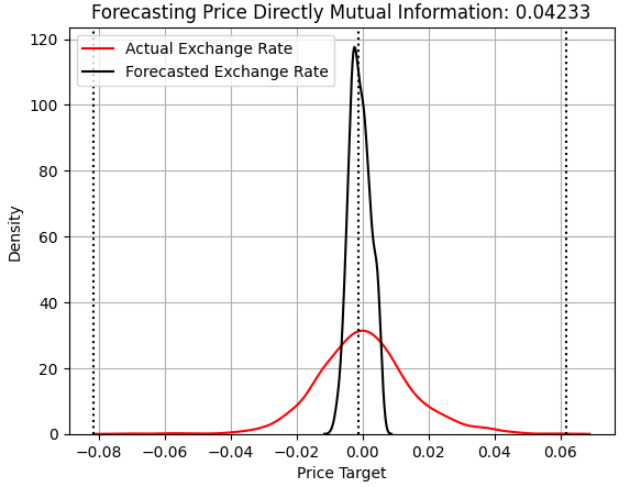
Figure 1: Visualizing our model's predictions against the real exchange rates observed out of sample when forecasting price

In the scatterplot, the problem becomes even clearer. The model’s predictions (in black) lie along the middle of the real exchange rates (in red). This is the reward hacking issue we introduced earlier. Traditional “best practices” would favor RMSE and thus encourage using this model in live trading. But as we’ll see, MI catches this problem quickly and provides a more robust performance measure.

plt.scatter(x=np.arange(y_test.shape[0]),y=y_test.iloc[:,0],color='red')
plt.scatter(x=np.arange(y_test.shape[0]),y=preds_a,color='black')
plt.legend(['Actual Exchange Rate','Forecasted Exchange Rate'])
plt.xlabel('Historical Time Epochs')
plt.ylabel('EURUSD Exchange Rate')
plt.title(s)
plt.grid()

Figure 2: Our first model is demonstrating mean-hugging behavior which is undesirable

Let us now consider the performance of a statistical model learning to expect changes in the Close Moving Average indicator. The same style of presentation is used throughout our graphs, so we can quickly observe that this model still fails to capture the width of the target—though its MI score has increased by more than 100%, from 0.04 to 0.1. However, Figure 3’s KDE plot doesn’t make it obvious why the MI score improved.

score_2 =  mutual_info_regression(y_test.iloc[:,[1]],preds_b)
score_2_rmse =  root_mean_squared_error(y_test.iloc[:,[1]],preds_b)
s = 'Forecasting Moving Average Directly Mutual Information: ' + str(score_2[0])[:7]
plt.title(s)
sns.kdeplot(y_test.iloc[:,1],color='red')
sns.kdeplot(preds_b,color='black')
plt.axvline(y.iloc[:,1].mean(),color='black',linestyle=':')
plt.axvline(y.iloc[:,1].max(),color='black',linestyle=':')
plt.axvline(y.iloc[:,1].min(),color='black',linestyle=':')
plt.legend(['Actual Moving Average','Forecasted Moving Average'])
plt.grid()

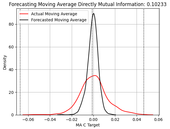
Figure 3: Visualizing our ability to forecast changes in the Close Moving Average Indicator

The improvement becomes clear when we examine a scatterplot of the model’s out-of-sample predictions. What was once a thin black line centered on the observed exchange rates has now widened into a more spread-out distribution, showing increased sensitivity to changes in the EURUSD market. The model is still not acceptable, but it is a step in the right direction.

plt.scatter(x=np.arange(y_test.shape[0]),y=y_test.iloc[:,1],color='red')
plt.scatter(x=np.arange(y_test.shape[0]),y=preds_b,color='black')
plt.legend(['Actual Moving Average','Forecasted Moving Average'])
plt.xlabel('Historical Time Epochs')
plt.ylabel('EURUSD Moving Average')
plt.title(s)
plt.grid()

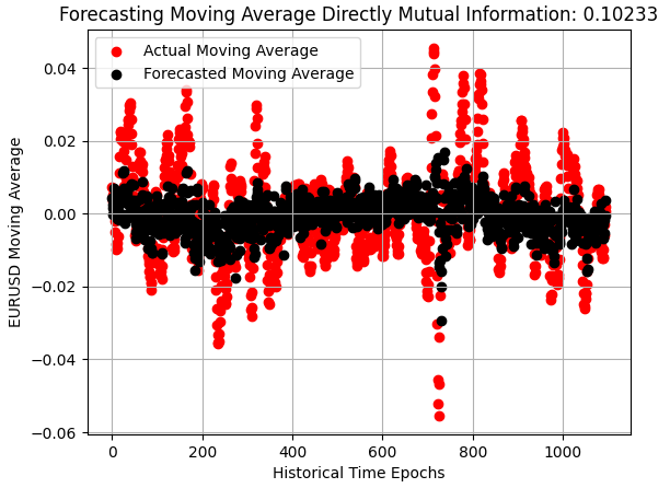
Figure 4: Our model has improved materially and is starting to capture the volatility of the market

When we evaluate the model forecasting the Stochastic indicator, we see material improvements. Even before considering the dramatic increase in MI, we can see we’ve finally produced a model that does not hug the mean. This model is the only one in our discussion that reasonably resembles the distribution of test observations and captures the market’s width better than the prior models.

score_3 = mutual_info_regression(y_test.iloc[:,[2]],preds_c)
score_3_rmse = root_mean_squared_error(y_test.iloc[:,[2]],preds_c)
s = 'Forecasting EURUSD Stochastic Directly MI: ' + str(score_3[0])[:7]
plt.title(s)
sns.kdeplot(y_test.iloc[:,2],color='red')
sns.kdeplot(preds_c,color='black')
plt.axvline(y.iloc[:,2].mean(),color='black',linestyle=':')
plt.axvline(y.iloc[:,2].max(),color='black',linestyle=':')
plt.axvline(y.iloc[:,2].min(),color='black',linestyle=':')
plt.legend(['Actual Stochastic','Forecasted Stochastic'])
plt.grid()

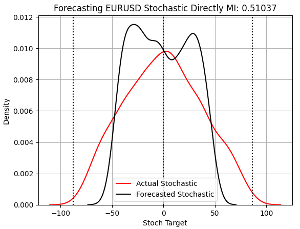
Figure 5: Our model is finally producing results that are symmetrical to the true observations that we kept out of training

Additionally, when we examine a scatterplot of the results, the reason for the dramatic jump in MI becomes clear. The Stochastic model performs impressively out of sample and nearly captures the true volatility of the market. By comparing this scatterplot to Figure 1, it becomes evident why MI is a strong candidate for automatically selecting regression targets.

plt.scatter(x=np.arange(y_test.shape[0]),y=y_test.iloc[:,2],color='red')
plt.scatter(x=np.arange(y_test.shape[0]),y=preds_c,color='black')
plt.ylabel('Growth in The Stochastic Main Indicator')
plt.xlabel('Historical Time Epochs')
plt.title(s)
plt.grid()

Figure 6: Visualizing our ability to capture changes in the Stochastic Oscilator

Next, we consider forecasting the RSI and its associated changes. Unfortunately, as shown below, the RSI is as challenging to forecast as the moving average indicators and brings the MI score back down to where it was earlier. The model also fails to capture the true width of the market, although the test set’s RSI changes do naturally cluster around 0. However, the model overestimates this proportion, potentially leading to suboptimal performance.

score_4 = mutual_info_regression(y_test.iloc[:,[3]],preds_d)
score_4_rmse = root_mean_squared_error(y_test.iloc[:,[3]],preds_d)
s = 'Forecasting EURUSD RSI Directly MI: ' + str(score_4[0])[:7]
plt.title(s)
sns.kdeplot(y_test.iloc[:,3],color='red')
sns.kdeplot(preds_d,color='black')
plt.axvline(y.iloc[:,3].mean(),color='black',linestyle=':')
plt.axvline(y.iloc[:,3].max(),color='black',linestyle=':')
plt.axvline(y.iloc[:,3].min(),color='black',linestyle=':')
plt.grid()
plt.legend(['Actual RSI','Forecasted RSI'])

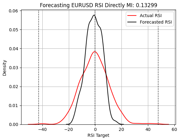
Figure 7: Our RSI strategy appears to be overestimating the number of predictions clustered around 0

Finally, when we examine the RSI forecast scatterplot, we can see that while this model is better than the mean-hugging model we started with—it doesn’t just run along the center of the observations—it still fails to capture the market dynamics as well as the Stochastic oscillator model.

plt.scatter(x=np.arange(y_test.shape[0]),y=y_test.iloc[:,3],color='red')
plt.scatter(x=np.arange(y_test.shape[0]),y=preds_d,color='black')
plt.legend(['Actual RSI','Forecasted RSI'])
plt.xlabel('Historical Time Epochs')
plt.ylabel('EURUSD Moving Average')
plt.title('Visualizing Our Ability To Forecast Change in EURUSD Moving Average')
plt.grid()

Figure 8: Our strategy performed better at learning to expect changes in the RSI, than changes in Price directly

From everything we’ve seen, it should be clear that the model learning to predict changes in the Stochastic oscillator performs best, even out of sample. We could recognize this visually from the scatterplots. Now, after creating a bar plot of MI scores for each target, we see a clear winner. But the reader should note, we’ve arrived at the heart of the problem this article addresses. We plotted the MI scores for each model, but we also recorded their RMSE scores. What happens when we instead plot RMSE?

mi_scores   = [score_1,score_2,score_3,score_4]
rmse_scores = [score_1_rmse,score_2_rmse,score_3_rmse,score_4_rmse]

sns.barplot(mi_scores,color='black')
plt.ylabel('Mutual Information Score')
plt.xlabel('Target')
plt.title('Mutual Information Score')
plt.xticks([0,1,2,3],['Price','Moving Average','Stochastic','RSI'])

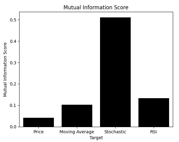
Figure 9: Mutual Information correctly identifies the appropriate target for us to model because it is not sensitive to the scale of the data

As shown, RMSE—the metric many practitioners rely upon—tells a completely different story. Remember, RMSE and MI are interpreted differently. When using MI, we want models that maximize the score. With RMSE, we want to minimize the score. Unfortunately, RMSE would lead us to pick the Price or Moving Average models, even though we visually confirmed they were suboptimal.

Given all the information you have read so far, would you trust RMSE or MI to guide you? Some readers may now clearly see the problem. But for those still unsure, we include one more test to expose the weakness of RMSE. 

sns.barplot(rmse_scores,color='black')
plt.xticks([0,1,2,3],['Price','Moving Average','Stochastic','RSI'])
plt.title('RMSE Score ')
plt.ylabel('Root Mean Squared Error')
plt.xlabel('Target')

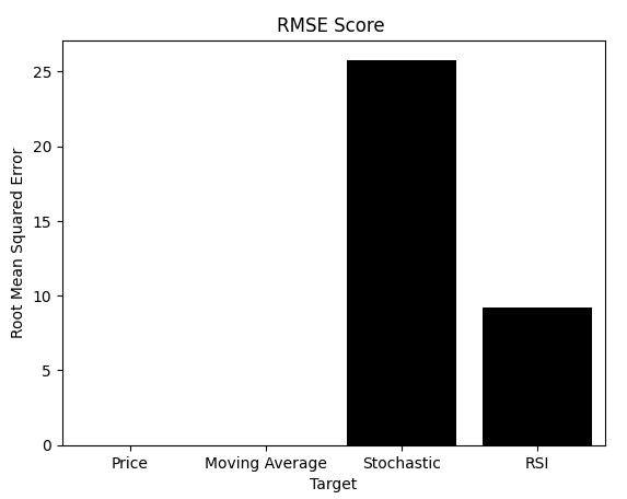
Figure 10: RMSE could incorrectly lead us to believe that the model learning the Stochastic oscillator is performing poorly

We again redefine a method to produce a fresh classifier model and compare its accuracy when classifying binary changes in each target. As before, we create four identical copies of the same model and measure cross-validation accuracy on the training set. We also tracked the accuracy each model would obtain by simply predicting the majority class in its training set—another form of reward hacking to watch for. When we plot these results, the truth becomes clear: the Stochastic model is the best performer, just as MI clearly revealed earlier. The red line in the plot shows the highest accuracy any model could achieve through reward hacking, confirming that the Stochastic model’s performance is legitimately significant.

def get_model():
    return(AdaBoostClassifier())

#Control model
model_a = get_model()

#Close Moving Average model
model_b = get_model()

#Stoch model
model_c = get_model()

#RSI model
model_d = get_model()

score   = []

score.append(np.mean(cross_val_score(model_a,X,y_classif.iloc[:,0],cv=tscv,scoring='accuracy',n_jobs=-1)))
score.append(np.mean(cross_val_score(model_b,X,y_classif.iloc[:,1],cv=tscv,scoring='accuracy',n_jobs=-1)))
score.append(np.mean(cross_val_score(model_c,X,y_classif.iloc[:,2],cv=tscv,scoring='accuracy',n_jobs=-1)))
score.append(np.mean(cross_val_score(model_d,X,y_classif.iloc[:,3],cv=tscv,scoring='accuracy',n_jobs=-1)))

h1 = y_classif.loc[y_classif['Price Target 2'] == 1].shape[0] / y_classif.shape[0]
h2 = y_classif.loc[y_classif['MA C Target 2'] == 1].shape[0] / y_classif.shape[0]
h3 = y_classif.loc[y_classif['Stoch Target 2'] == 1].shape[0] / y_classif.shape[0]
h4 = y_classif.loc[y_classif['RSI Target 2'] == 1].shape[0] / y_classif.shape[0]

reward_hacking = [h1,h2,h3,h4]

sns.barplot(score,color='black')
plt.xticks([0,1,2,3],['Price','MA','Stochastic','RSI'])
plt.ylabel('Accuracy Score 100%')
plt.xlabel('Potential Target')
plt.axhline(np.max(reward_hacking),color='red',linestyle=':')
plt.title('Our Accuracy Changes Depending On The Target')

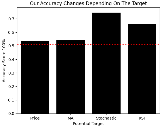
Figure 11: Even when we set up our problem as a classification task, we arrive at the same conclusion

Now that we have identified the strategy our black-box model learns best, we can derive trading rules directly from the data. For instance, if the stochastic oscillator is predicted to increase, should we go long or short? One way to answer this is by examining the average return across all instances where the stochastic had a label of 1. In our case, that average was 0.0052, suggesting it is reasonable to enter long positions when the oscillator is expected to rise.

data.loc[data['Stoch Target 2']==1,'Price Target'].mean()

0.005242425488180883

Of course, no strategy is perfect—there were instances where price fell despite a positive label. 

data.loc[data['Stoch Target 2']==1,'Price Target'].min()

-0.06370000000000009

However, the value of this exercise is that it allows the reader to assess whether the strategy aligns with their risk profile using data rather than intuition. By calculating how often price and the stochastic oscillator moved together, we find they aligned 71% of the time. This prior gives us further confidence in this strategy.

print('Price And The Stochastic Rise Together: ',((data.loc[(data['Stoch Target 2']==1 ) & (data['Price Target 2']==1),:].shape[0] / data.loc[data['Price Target 2'] == 1].shape[0])) * 100,'% of the time')

Price And The Stochastic Rise Together:  70.94972067039106 % of the time

If even simple models can recognize that the stochastic oscillator is easier to learn, then a more flexible model like a deep neural network, properly configured, should capture this relationship even better. We’ll explore this by performing a randomized search over neural network hyperparameters. First, we list all possible input values to evaluate. 

dist = {
    'max_iter':[10,50,100,500,1000,5000,10000,50000,100000],
    'activation':['tanh','relu','identity','logistic'],
    'alpha':[10e0,10e-1,10e-2,10e-3,10e-4,10-5,10e-6],
    'solver':['lbfgs','adam','sgd'],
    'learning_rate':['constant','invscaling','adaptive'],
    'hidden_layer_sizes':[(11,1),(11,22,33,44,33,22,11,5),(11,4,40,20,2),(11,11),(11,11,11),(11,11,11,11),(11,22,33,44),(11,22,55,22,11),(11,100,11),(11,5,2,5,11),(11,3,9,18,9,3)]
}

Then, we define fixed constants that will remain unchanged during training.

#Define the model
model = MLPRegressor(shuffle=False,early_stopping=False,random_state=0,verbose=True)

#Initialize the randomized search object
rscv = RandomizedSearchCV(model,dist,random_state=0,n_iter=40,scoring='neg_mean_squared_error',cv=tscv,n_jobs=-1,refit=True)

#Perform the search
res = rscv.fit(X,y_classif['Stoch Target 2'])
res.best_estimator_

After selecting the best model via the random search, we are ready to export it to the ONNX (Open Neural Network Exchange) format. ONNX is a widely used open standard that makes models portable and framework-independent. We start by defining the input and output shapes expected by the model.

initial_types = [('float_input',FloatTensorType([1,X.shape[1]]))]
final_types   = [('float_output',FloatTensorType([1,1]))]

Next, we convert the ONNX model into its prototype form, which acts as an intermediate representation before saving it to disk using the ONNX save function.

onnx_proto = convert_sklearn(model=res.best_estimator_,initial_types=initial_types,final_types=final_types,target_opset=12)
onnx.save(onnx_proto,'Unsupervised Strategy Selection Stochastic MLP.onnx')

Building Our Application In MQL5

With the model ready, we can begin building our trading application. We start by loading the ONNX model and specifying system constants to ensure consistent indicator calculations across data retrieval and strategy selection.

//+------------------------------------------------------------------+
//|                                 Automatic Strategy Selection.mq5 |
//|                                               Gamuchirai Ndawana |
//|                    https://www.mql5.com/en/users/gamuchiraindawa |
//+------------------------------------------------------------------+
#property copyright "Gamuchirai Ndawana"
#property link      "https://www.mql5.com/en/users/gamuchiraindawa"
#property version   "1.00"

//+------------------------------------------------------------------+
//| System resources                                                 |
//+------------------------------------------------------------------+
#resource "\\Files\\Unsupervised Strategy Selection Stochastic MLP.onnx" as const uchar onnx_buffer[];

Next, we define system constants to ensure that the calculation of our technical indicators is consistent with both the data-fetching script and the indicator calculations from our earlier conversation on automatic strategy selection.

//+------------------------------------------------------------------+
//| System definiyions                                               |
//+------------------------------------------------------------------+
#define MA_PERIOD     5                    //--- Moving Average Period
#define MA_TYPE       MODE_SMA             //--- Type of moving average 
#define RSI_PERIOD    15                   //--- RSI Period
#define STOCH_K       5                    //--- Stochastich K Period
#define STOCH_D       3                    //--- Stochastich D Period
#define STOCH_SLOWING 3                    //--- Stochastic slowing
#define STOCH_MODE    MODE_EMA             //--- Stochastic mode
#define STOCH_PRICE   STO_LOWHIGH          //--- Stochastic price feeds
#define TOTAL_STRATEGIES 4                 //--- Total strategies we have to choose from
#define ONNX_INPUTS 11                     //--- Total inputs needed by our ONNX model
#define ONNX_OUTPUTS 1                     //--- Total outputs needed by our ONNX model

We will also need the trade library to help manage our market exposure.

//+------------------------------------------------------------------+
//| System libraries                                                 |
//+------------------------------------------------------------------+
#include <Trade\Trade.mqh>
CTrade Trade;

A handful of global variables will be necessary to keep track of time, indicator readings, and our model predictions.

//+------------------------------------------------------------------+
//| Global variables                                                 |
//+------------------------------------------------------------------+
int ma_c_handle,ma_o_handle,ma_h_handle,ma_l_handle,rsi_handle,stoch_handle,atr_handle;
double ma_c_reading[],ma_o_reading[],ma_h_reading[],ma_l_reading[],rsi_reading[],sto_reading_main[],sto_reading_signal[],atr_reading[];
long onnx_model;
vectorf onnx_features,onnx_targets;

MqlDateTime ts,tc;
MqlTick     current_tick;       

We can now initialize our ONNX model by creating it from the ONNX buffer using the OnnxCreateFromBuffer method. We then define and test the input and output dimensions and perform a final check to ensure the model is sound. If all tests pass, we initialize time tracking and the necessary technical indicators.

//+------------------------------------------------------------------+
//| Expert initialization function                                   |
//+------------------------------------------------------------------+
int OnInit()
  {
//--- Prepare the model's inputs and outputs
   onnx_features = vectorf::Zeros(ONNX_INPUTS);
   onnx_targets  = vectorf::Zeros(ONNX_OUTPUTS);

//--- Create the ONNX model
   onnx_model = OnnxCreateFromBuffer(onnx_buffer,ONNX_DATA_TYPE_FLOAT);

//--- Define the I/O shape
   ulong input_shape[] = {1,ONNX_INPUTS};
   ulong output_shape[] = {ONNX_OUTPUTS,1};

   if(!OnnxSetInputShape(onnx_model,0,input_shape))
     {
      Print("Failed to define ONNX input shape");
      return(INIT_FAILED);
     }

   if(!OnnxSetOutputShape(onnx_model,0,output_shape))
     {
      Print("Failed to define ONNX output shape");
      return(INIT_FAILED);
     }

//--- Check if the model is valid
   if(onnx_model == INVALID_HANDLE)
     {
      Print("Failed to create our ONNX model from buffer");
      return(INIT_FAILED);
     }

//--- Setup the time
   TimeLocal(tc);
   TimeLocal(ts);

//---Setup our technical indicators
   ma_c_handle = iMA(_Symbol,PERIOD_CURRENT,MA_PERIOD,0,MA_TYPE,PRICE_CLOSE);
   ma_o_handle = iMA(_Symbol,PERIOD_CURRENT,MA_PERIOD,0,MA_TYPE,PRICE_OPEN);
   ma_h_handle = iMA(_Symbol,PERIOD_CURRENT,MA_PERIOD,0,MA_TYPE,PRICE_HIGH);
   ma_l_handle = iMA(_Symbol,PERIOD_CURRENT,MA_PERIOD,0,MA_TYPE,PRICE_LOW);
   atr_handle = iATR(_Symbol,PERIOD_CURRENT,14);
   rsi_handle  = iRSI(_Symbol,PERIOD_CURRENT,RSI_PERIOD,PRICE_CLOSE);
   stoch_handle = iStochastic(_Symbol,PERIOD_CURRENT,STOCH_K,STOCH_D,STOCH_SLOWING,STOCH_MODE,STOCH_PRICE);
//---
   return(INIT_SUCCEEDED);
  }

If the application is no longer in use, we will free the resources assigned to the ONNX model and technical indicators.

//+------------------------------------------------------------------+
//| Expert deinitialization function                                 |
//+------------------------------------------------------------------+
void OnDeinit(const int reason)
  {
//---
   OnnxRelease(onnx_model);
   IndicatorRelease(ma_c_handle);
   IndicatorRelease(ma_o_handle);
   IndicatorRelease(ma_h_handle);
   IndicatorRelease(ma_l_handle);
   IndicatorRelease(rsi_handle);
   IndicatorRelease(stoch_handle);
   IndicatorRelease(atr_handle);
  }

Whenever new price levels are received, we will first check if a new daily candle has formed, then update the time and all technical indicator readings. Each model input is then cast to a float to ensure compatibility with the ONNX model before generating a prediction. The prediction is compared against our market entry conditions to determine the appropriate position.

//+------------------------------------------------------------------+
//| Expert tick function                                             |
//+------------------------------------------------------------------+
void OnTick()
  {
//---
   TimeLocal(ts);

   if(ts.day != tc.day)
     {
      //--- Update the time
      TimeLocal(tc);

      //--- Update Our indicator readings
      CopyBuffer(ma_c_handle,0,0,1,ma_c_reading);
      CopyBuffer(ma_o_handle,0,0,1,ma_o_reading);
      CopyBuffer(ma_h_handle,0,0,1,ma_h_reading);
      CopyBuffer(ma_l_handle,0,0,1,ma_l_reading);
      CopyBuffer(rsi_handle,0,0,1,rsi_reading);
      CopyBuffer(stoch_handle,0,0,1,sto_reading_main);
      CopyBuffer(stoch_handle,0,0,1,sto_reading_signal);
      CopyBuffer(atr_handle,0,0,1,atr_reading);

      //--- Set our model inputs
      onnx_features[0] = (float) iOpen(Symbol(),PERIOD_CURRENT,0);
      onnx_features[1] = (float) iHigh(Symbol(),PERIOD_CURRENT,0);
      onnx_features[2] = (float) iLow(Symbol(),PERIOD_CURRENT,0);
      onnx_features[3] = (float) iClose(Symbol(),PERIOD_CURRENT,0);
      onnx_features[4] = (float) ma_o_reading[0];
      onnx_features[5] = (float) ma_h_reading[0];
      onnx_features[6] = (float) ma_l_reading[0];
      onnx_features[7] = (float) ma_c_reading[0];
      onnx_features[8] = (float) rsi_reading[0];
      onnx_features[9] = (float)  sto_reading_main[0];
      onnx_features[10] = (float) sto_reading_signal[0];

      //--- Copy Market Data
      double close = iClose(Symbol(),PERIOD_CURRENT,0);
      SymbolInfoTick(Symbol(),current_tick);

      //--- Place a position
      if(PositionsTotal() ==0)
        {
         if(OnnxRun(onnx_model,ONNX_DATA_TYPE_FLOAT,onnx_features,onnx_targets))
           {
            Comment("Onnx Model Prediction: \n",onnx_targets);

            //--- Store our result
            if(LongConditions())
               Buy();

            else
               if(ShortConditions())
                  Sell();
           }
         else
           {
            Print("No trading oppurtunities expected.");
           }
        }
     }
  }
//+------------------------------------------------------------------+

Our market entry conditions are defined in their own dedicated methods. If the ONNX prediction exceeds 0.5, the stochastic oscillator is expected to rise. If the oscillator is above 50 and still rising, we take a long position. Alternatively, if the oscillator is below the classical 30 level, we also enter long positions. Finally, if we observe a bullish engulfing candle, this is our last condition to go long. The opposite holds true for short entries.

//+------------------------------------------------------------------+
//| The market conditions we require to open short positions         |
//+------------------------------------------------------------------+
bool ShortConditions(void)
  {
   return(((onnx_targets[0] < 0.5) && (sto_reading_main[0]<50)) || (sto_reading_main[0]<80) || (iHigh(Symbol(),PERIOD_CURRENT,1) > iHigh(Symbol(),PERIOD_CURRENT,2) && iLow(Symbol(),PERIOD_CURRENT,1) > iLow(Symbol(),PERIOD_CURRENT,2) && iOpen(Symbol(),PERIOD_CURRENT,1)<iOpen(Symbol(),PERIOD_CURRENT,2)));
  }

//+------------------------------------------------------------------+
//| The market conditions we require to open long positions          |
//+------------------------------------------------------------------+
bool LongConditions(void)
  {
   return(((onnx_targets[0] > 0.5) && (sto_reading_main[0]>50)) || (sto_reading_main[0]>30) || (iHigh(Symbol(),PERIOD_CURRENT,1) > iHigh(Symbol(),PERIOD_CURRENT,2) && iLow(Symbol(),PERIOD_CURRENT,1) > iLow(Symbol(),PERIOD_CURRENT,2) && iOpen(Symbol(),PERIOD_CURRENT,1)>iOpen(Symbol(),PERIOD_CURRENT,2)));
  }

When placing positions, whether long or short, we will use the same lot size for each entry and set equally spaced take-profit and stop-loss levels.

//+------------------------------------------------------------------+
//| Enter a long position                                            |
//+------------------------------------------------------------------+
void Buy(void)
  {
   Trade.Buy(0.01,Symbol(),current_tick.ask,current_tick.ask-(1.5*atr_reading[0]),current_tick.ask+(1.5*atr_reading[0]));
  }

//+------------------------------------------------------------------+
//| Enter a short position                                           |
//+------------------------------------------------------------------+
void Sell(void)
  {
   Trade.Sell(0.01,Symbol(),current_tick.bid,current_tick.bid+(1.5*atr_reading[0]),current_tick.bid-(1.5*atr_reading[0]));
  }
//+------------------------------------------------------------------+

Finally, we undefine all system constants at the end of each application.

//+------------------------------------------------------------------+
//| Undefine system constants                                        |
//+------------------------------------------------------------------+
#undef MA_PERIOD
#undef MA_TYPE
#undef RSI_PERIOD
#undef STOCH_K
#undef STOCH_D
#undef STOCH_SLOWING
#undef STOCH_MODE
#undef STOCH_PRICE
#undef TOTAL_STRATEGIES
#undef ONNX_INPUTS
#undef ONNX_OUTPUTS
//+------------------------------------------------------------------+

With the setup of our application complete, we will now select the 3-year backtest window that we kept out of our model training earlier in the conversation. The backtest will span from January 2022 to well past January 2025.

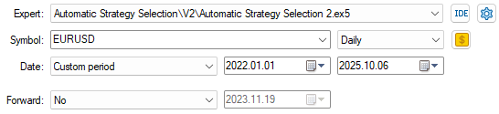
Figure 12: Selecting the backtest window to evaluate our strategy over

Using modeling based on real ticks with random delay settings gives a reliable emulation of real market conditions.

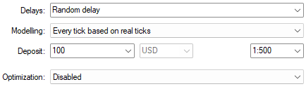
Figure 13: Select the right backtest conditions to learn realistic expectations

The equity curve produced by our revised black-box solution shows a strong uptrend, demonstrating strategy health. We also observe periods where the strategy was challenged, but we are encouraged to see that it recovered from each drawdown with resilience.

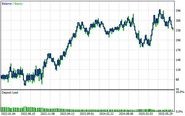
Figure 14: Visualizing the equity curve we obtained by following our carefully revised trading strategy gives us confidence in the changes we made

Finally, when we analyze the detailed statistics of our strategy, we observe significant improvement compared to our first attempt to model all possible strategies. Our strategy was profitable, with a strong recovery and profit factor.

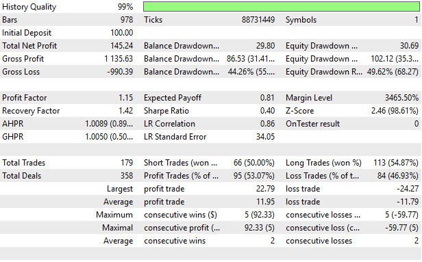
Figure 15: Visualizing the detailed results produced by our improved black-box solution

Conclusion

We have now arrived at the end of our discussion. This article presented the reader with a careful demonstration of how to configure any black-box solution to automatically identify good strategies. In our previous discussion, we attempted to model all possible strategies and then only take signals from the strategy expected to be most profitable, producing a profit of $38.58 during that backtest. In this discussion, we have proposed how Mutual Information can be used to quickly identify the best strategy for our statistical estimator to learn, improving profit levels to $145.24 over the same backtest period, with all other variables, such as position sizing and trading volume, held constant.

Our proposed solution today improved our Sharpe Ratio from 0.13 initially to 0.4. This article has taught the reader how to carefully configure your black-box solution using the numerical techniques discussed, and, most importantly, how to avoid the blind spots of conventional “best practices” such as overreliance on RMSE for cross-validating regression models and its tendency to reward mean-hugging behavior in models.