Neural Networks in Trading: Models Using Wavelet Transform and Multi-Task Attention

Introduction

Asset return prediction is a widely studied topic in finance. The challenge of forecasting returns arises due to several factors. First, the multitude of variables influencing asset returns and the low signal-to-noise ratio in large, sparse matrices make it difficult to extract meaningful information using traditional econometric models. Second, the functional relationships between predictive features and asset returns remain unclear, posing challenges in capturing the nonlinear structures among them.

In recent years, deep learning has become an indispensable tool in quantitative investing, particularly in refining multifactor strategies that form the foundation for understanding financial asset price movements. By automating feature learning and capturing nonlinear relationships in financial market data, deep learning algorithms effectively uncover complex patterns, thereby improving prediction accuracy. The global research community recognizes the potential of deep neural networks, such as recurrent neural networks (RNNs) and convolutional neural networks (CNNs), for forecasting stock and futures prices. However, while RNNs and CNNs are widely used, deeper neural architectures that extract and construct sequential market and signal information remain underexplored. This opens opportunities for further advancements in applying deep learning to stock markets.

Today, we introduce the Multitask-Stockformer framework, presented in the paper "Stockformer: A Price-Volume Factor Stock Selection Model Based on Wavelet Transform and Multi-Task Self-Attention Networks". Despite the similarity in name to the previously discussed StockFormer framework, these two models are unrelated - except for their shared objective: generating a profitable stock portfolio for trading in financial markets.

The Multitask-Stockformer framework builds a multi-task stock forecasting model based on wavelet transform and self-attention mechanisms.

The Multitask-Stockformer Algorithm

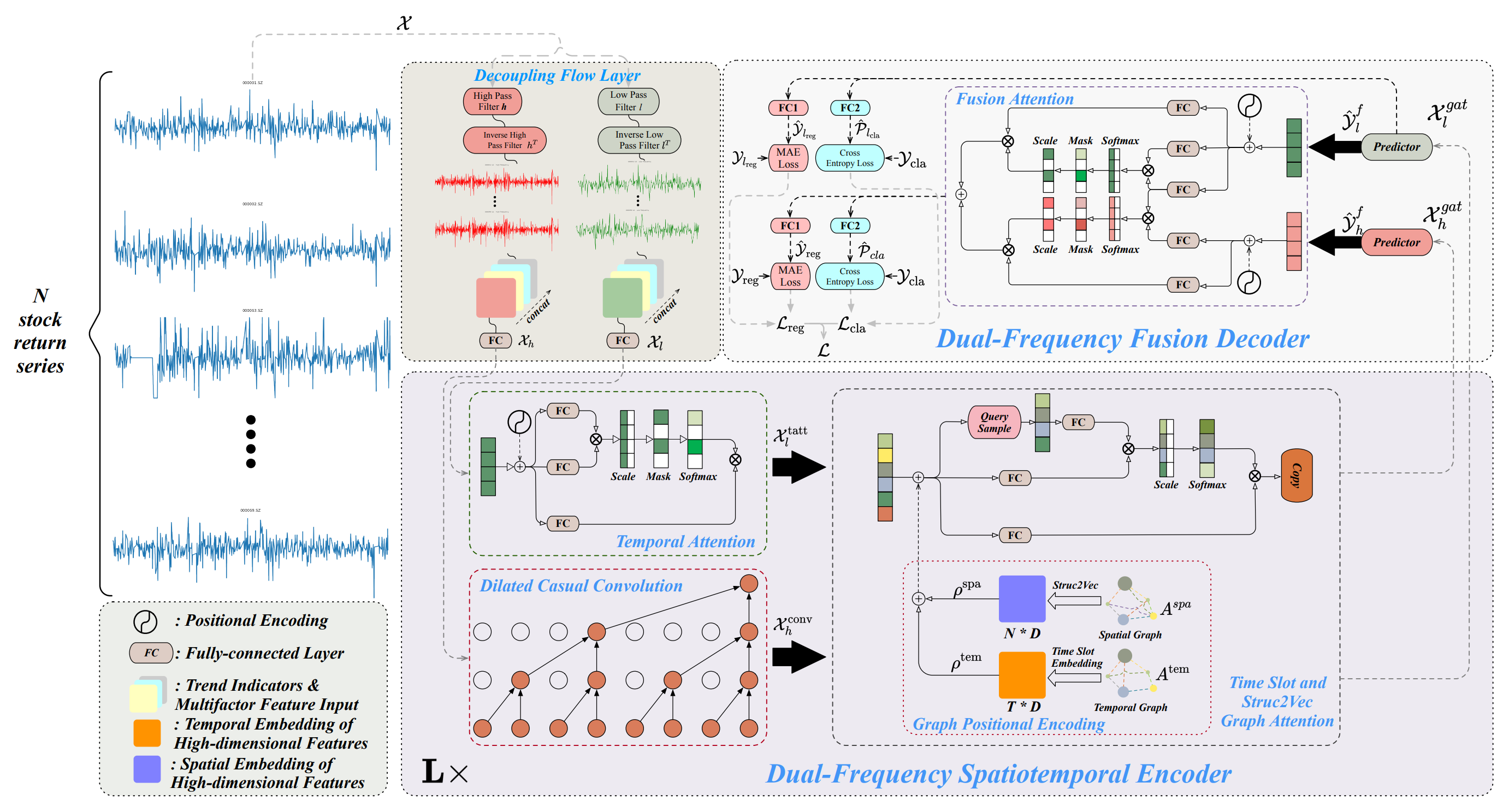
The architecture of the Multitask-Stockformer framework is divided into three modules: a flow separation module, a dual-frequency spatiotemporal encoder, and a dual-frequency decoder. The analyzed historical asset data 𝒳 ∈ RT1×N×362 is processed in the flow separation module. At this stage, the asset return tensor is decomposed into high- and low-frequency components using a discrete wavelet transform, while trend features and price-volume ratios remain unchanged. These components are then concatenated with the unchanged parts of the signal along the last dimension.

The low-frequency component represents long-term trends, while the high-frequency component captures short-term fluctuations and sharp events. These are denoted as 𝒳l, 𝒳h ∈ RT1×N×362, respectively. Next, both 𝒳h and 𝒳l linearly transformed through a fully connected layer into the dimension RT1×N×D. Here T1 denotes the depth of the historical data analyzed.

The dual-frequency spatiotemporal encoder is designed to represent these different time series patterns: low-frequency features are fed into a temporal attention module (denoted as tatt), while high-frequency features are processed through an extended causal convolutional layer (denoted as conv). These outputs are then input into graph attention networks (denoted as gat). Interaction with graph-based information allows the model to capture complex relationships and dependencies between assets and time. In this module, the spatial graph Aspa and temporal graph Atem are transformed via fully connected layers and tensor translation operations into multidimensional embeddings, denoted ρspa, ρtem ∈ RT1×N×D, which are then combined with 𝒳l,tatt, 𝒳h,conv using addition and graph attention operations to produce 𝒳l,gat, 𝒳h,gat ∈ RT1×N×D. The dual-frequency spatiotemporal encoder consists of L layers aimed at efficiently representing multi-scale spatiotemporal patterns of low- and high-frequency waves. Finally, in the dual-frequency decoder, predictors generate 𝒴l,f, 𝒴h,f ∈ RT2×N×D, which are aggregated using Fusion Attention interactions to obtain a latent representation of two-scale temporal patterns. Separate fully connected layers (a regression layer, FC1, and a classification layer, FC2) produce multi-task outputs, including stock return forecasts (the regression output, denoted reg) and stock trend prediction probabilities (the classification output, denoted cla).

Additionally, regression values and trend prediction probabilities are derived for the low-frequency component, improving the learning process of the low-frequency signal.

An author-provided visualization of the Multitask-Stockformer framework is shown below.

Implementation in MQL5

Above is only a brief description of the Multitask-Stockformer framework. The framework is fairly complex. I believe it will be more effective to become familiar with its individual algorithms during their implementation. We will begin work with the flow-separation module of the raw data.

Signal decomposition module

To split the analyzed signal into low-frequency and high-frequency components, the framework's authors propose using the discrete wavelet transform. Unlike the Fourier decomposition, the wavelet transform is capable of capturing not only the frequency content but also the structure of the signal. This makes it more advantageous for financial market analysis, where not only frequency but also the ordering of signals is important.

Previously, we already used the discrete wavelet transform when building the FEDformer framework, but then we extracted only the low-frequency component. Now we need the high-frequency component as well. Nevertheless, we can reuse existing developments.

The discrete wavelet transform is, in essence, a convolution operation with a certain wavelet used as the filter. This allows us to use convolutional layer algorithms as the base functionality. It should be noted that in the transformation we use static wavelets whose parameters do not change during training. Therefore, we must disable the optimization mechanism for our object's parameters.

With the above in mind, we create a new object for extracting high- and low-frequency signal components using the discrete wavelet transform CNeuronLegendreWaveletsHL.

class CNeuronLegendreWaveletsHL :  public CNeuronConvOCL
  {
protected:
   virtual bool      updateInputWeights(CNeuronBaseOCL *NeuronOCL)   { return true; }

public:
                     CNeuronLegendreWaveletsHL(void) {};
                    ~CNeuronLegendreWaveletsHL(void) {};
   virtual bool      Init(uint numOutputs, uint myIndex, COpenCLMy *open_cl, 
                          uint window, uint step, uint units_count, 
                          uint filters, uint variables, 
                          ENUM_OPTIMIZATION optimization_type, uint batch) override;
   //---
   virtual int       Type(void)   const   {  return defNeuronLegendreWaveletsHL;   }
   //---
   virtual uint      GetFilters(void)  const {return (iWindowOut / 2); }
   virtual uint      GetVariables(void)  const {return (iVariables); }
   virtual uint      GetUnits(void)  const {return (Neurons() / (iVariables * iWindowOut)); }
  };

As already mentioned, the discrete wavelet transform is a convolution with a wavelet filter. This allows us to fully leverage the parent convolution layer class functionality when building the algorithm. It is sufficient to override the initialization method, replacing the random filter parameters with the wavelet data.

However, the wavelet filters used are static. Therefore, we override the parameter optimization method updateInputWeights with a no-op implementation.

Initialization of the new object is performed in the Init method. As usual, this method receives from the external program a set of constants that uniquely identify the architecture of the object being created. These include:

• window — the size of the analysis window;
• step — the step of the analysis window;
• units_count — the number of convolution operations per single sequence;
• filters — the number of filters used;
• variables — the number of single sequences in the analyzed multimodal time series. 

bool CNeuronLegendreWaveletsHL::Init(uint numOutputs, uint myIndex, COpenCLMy *open_cl, 
                                     uint window, uint step, uint units_count, 
                                     uint filters, uint variables, 
                                     ENUM_OPTIMIZATION optimization_type, uint batch)
  {
   if(!CNeuronConvOCL::Init(numOutputs, myIndex, open_cl, window, step, 2 * filters, 
                                  units_count, variables, optimization_type, batch))
      return false;

Inside the method body, we immediately pass the received parameters to the parent class method of the same name. However, note that when calling the parent method we double the number of filters. This is due to the need to create filters for extracting both the low- and high-frequency components.

After the parent method completes successfully, we clear the convolution parameter buffer by filling it with zeros, and we define a constant offset in the buffer between elements of the low- and high-frequency filters.

   WeightsConv.BufferInit(WeightsConv.Total(), 0);
   const uint shift_hight = (iWindow + 1) * filters;

We then organize a system of nested loops to generate the required number of filters. Here we use a recursive generation of Legendre wavelets and sequentially fill the filter matrix with higher-order wavelets.

   for(uint i = 0; i < iWindow; i++)
     {
      uint shift = i;
      float k = float(2.0 * i - 1.0) / iWindow;
      for(uint f = 1; f <= filters; f++)
        {
         float value = 0;
         switch(f)
           {
            case 1:
               value = k;
               break;
            case 2:
               value = (3 * k * k - 1) / 2;
               break;
            default:
               value = ((2 * f - 1) * k * WeightsConv.At(shift - (iWindow + 1)) - 
                       (f - 1) * WeightsConv.At(shift - 2 * (iWindow + 1))) / f;
               break;
           }

For each element of the analysis window we create an inner loop to generate filter elements. In that loop we first generate the element of the corresponding low-frequency filter.

We then create another nested loop in which we propagate the generated element into the filters for all independent variables of the multimodal sequence. At the same time we add the high-frequency filter element, formed based on the corresponding low-frequency filter element.

         for(uint v = 0; v < iVariables; v++)
           {
            uint shift_var = 2 * shift_hight * v;
            if(!WeightsConv.Update(shift + shift_var, value))
               return false;
            if(!WeightsConv.Update(shift + shift_var + shift_hight, 
                                    MathPow(-1.0f, float(i))*value))
               return false;
           }

Then we adjust the offset to the next filter element and proceed to the next iteration of the looping system.

         shift += iWindow + 1;
        }
     }

The remainder of this initialization method differs from those we examined previously. Until now we have not used fragments of OpenCL code during object initialization. This method is an exception. Here we normalize the obtained wavelet filters.

   if(!!OpenCL)
     {
      if(!WeightsConv.BufferWrite())
         return false;
      uint global_work_size[] = {iWindowOut * iVariables};
      uint global_work_offset[] = {0};
      OpenCL.SetArgumentBuffer(def_k_NormilizeWeights, def_k_norm_buffer, WeightsConv.GetIndex());
      OpenCL.SetArgument(def_k_NormilizeWeights, def_k_norm_dimension, (int)iWindow + 1);
      if(!OpenCL.Execute(def_k_NormilizeWeights, 1, global_work_offset, global_work_size))
        {
         string error;
         CLGetInfoString(OpenCL.GetContext(), CL_ERROR_DESCRIPTION, error);
         printf("Error of execution kernel %s Normalize: %s", __FUNCSIG__, error);
         return false;
        }
     }
//---
   return true;
  }

After successfully normalizing the parameters, the method completes its execution, returning a Boolean result to the calling program.

The full code for the presented object and all its methods is available in the attachment.

It is worth noting that the functionality of the signal decomposition module extends beyond discrete wavelet transform, though this remains its core component. We plan to use the object in our models, where the input is a two-dimensional tensor of a multimodal time series with dimensions {Bar, Indicator Value}. For proper operation, the discrete wavelet transform requires transposition of the input data. This can be done externally before feeding the data into the object. But our goal is to build objects that are as user-friendly as possible. Therefore, we create a flow decomposition module object with slightly extended functionality, CNeuronDecouplingFlow, using the previously created discrete wavelet transform object as its parent class.

class CNeuronDecouplingFlow   :  public   CNeuronLegendreWaveletsHL
  {
protected:
   CNeuronTransposeOCL  cTranspose;
   //---
   virtual bool      feedForward(CNeuronBaseOCL *NeuronOCL);
   virtual bool      calcInputGradients(CNeuronBaseOCL *NeuronOCL);

public:
                     CNeuronDecouplingFlow(void) {};
                    ~CNeuronDecouplingFlow(void) {};
   virtual bool      Init(uint numOutputs, uint myIndex, COpenCLMy *open_cl,
                          uint window, uint step, uint units_count,
                          uint filters, uint variables,
                          ENUM_OPTIMIZATION optimization_type, uint batch);
   //---
   virtual int       Type(void)   const   {  return defNeuronDecouplingFlow;   }
   //---
   virtual bool      Save(int const file_handle) override;
   virtual bool      Load(int const file_handle) override;
   //---
   virtual void      SetOpenCL(COpenCLMy *obj) override;
  };

Within the new object, we add a data pre-transposition layer and redefine the external parameter units_count in the Init method to make it more user-friendly. Here, units_count represents the length of the analyzed sequence (the number of bars), while variables corresponds to the number of indicators analyzed.

Let's consider the implementation of this approach in the Init method. In the method body, we first recalculate the number of convolution operations for a single sequence based on the original sequence length, convolution window size, and step. We then call the parent class Init method with these adjusted parameters.

bool CNeuronDecouplingFlow::Init(uint numOutputs, uint myIndex, COpenCLMy *open_cl,
                                 uint window, uint step, uint units_count,
                                 uint filters, uint variables,
                                 ENUM_OPTIMIZATION optimization_type, uint batch)
  {
   uint units_out = (units_count - window + step) / step;
   if(!CNeuronLegendreWaveletsHL::Init(numOutputs, myIndex, open_cl, window, step, units_out, 
                                                filters, variables, optimization_type, batch))
      return false;

After successful execution of the parent method, we initialize the data transposition layer.

   if(!cTranspose.Init(0, 0, OpenCL, units_count, variables, optimization, iBatch))
      return false;
//---
   return true;
  }

The method ends by returning a logical result to the calling program.

The feed-forward and backpropagation algorithms are straightforward. For instance, in the forward pass, the input data are first transposed, and the resulting tensor is passed to the corresponding parent class method.

bool CNeuronDecouplingFlow::feedForward(CNeuronBaseOCL *NeuronOCL)
  {
   if(!cTranspose.FeedForward(NeuronOCL))
      return false;
   if(!CNeuronLegendreWaveletsHL::feedForward(cTranspose.AsObject()))
      return false;
//---
   return true;
  }

Therefore, we will not examine them in detail here. The full code for this object and all its methods is provided in the attachment.

Regarding the output of the signal decomposition module: the constructed operation flow does not allow the neural layer to return two separate tensors. Therefore, the results of the low- and high-frequency filters are output as a single tensor. Consequently, the output resembles a four-dimensional tensor {Variables, Units, [Low, High], Filters}. The separation into distinct data streams is planned for the dual-frequency spatiotemporal encoder.

After building the flow decomposition module, we proceed to implement the dual-frequency spatiotemporal encoder, which consists of three main components: temporal attention, dilated causal convolution, and a temporal slot with graph attention networks (Struc2Vec).

The authors of the Multitask-Stockformer framework organize two independent streams for low- and high-frequency components. These streams differ architecturally, allowing the model to focus on trends and seasonal components separately.

Low-frequency components are fed into the spatiotemporal attention block to capture long-term, low-frequency trends and global sequence relationships.

High-frequency components are processed by an expanded causal convolutional layer, focusing on local patterns, high-frequency fluctuations, and sudden events.

This dual-stream modeling approach is expected to improve the prediction accuracy of complex financial sequences.

For the spatiotemporal attention block, we can leverage existing Transformer-based encoder objects. The dilated causal convolution algorithm, however, requires custom implementation.

Dilated Causal Convolution Layer

The framework proposes an expanded causal convolution, a 1D convolution that skips input values at a defined step. Formally, for a sequence x ∈ RT and filter f ∈ RJ, the dilated causal convolution at time step t is defined as:

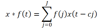
Here c is the dilation factor. The dilated causal convolution of the high-frequency component is expressed as:

In the original implementation, there is another hyperparameter - the dilation factor. It is constant. However, is the distance between dependent elements fixed throughout the sequence. Also, in the original algorithm, this factor is applied uniformly across different sequences.

In our implementation, we slightly modify this architecture. Instead of fixed skips, we introduce the Segment, Shuffle, Stitch (S3) algorithm, followed by a standard convolutional layer.

S3 allows the model to learn adaptive permutations of input segments, enabling the network to discover dependencies within high-frequency components. Stacking multiple S3 blocks further enhances the model's ability to capture complex high-frequency interactions.

We implement this approach in the object CNeuronDilatedCasualConv. The algorithm is linear. Therefore, we use the class CNeuronRMAT as the parent object, which provides the base functionality and interfaces for linear algorithm implementation. The structure of the new object is presented below.

class CNeuronDilatedCasualConv   :  public CNeuronRMAT
  {
public:
                     CNeuronDilatedCasualConv(void) {};
                    ~CNeuronDilatedCasualConv(void) {};
   //---
   virtual bool      Init(uint numOutputs, uint myIndex, COpenCLMy *open_cl,
                          uint window, uint step, uint dimension,
                          uint units_count, uint variables, uint layers,
                          ENUM_OPTIMIZATION optimization_type, uint batch);
   //---
   virtual int       Type(void) override   const   {  return defNeuronDilatedCasualConv; }
  };

As can be seen from the structure of the new object, choosing the "correct" parent class allows us to limit ourselves to specifying the object architecture in the Init method. All other functionality is already implemented in the parent class methods, which we inherit successfully.

In the Init method, we receive a set of constants from the external program, which uniquely define the architecture of the object being created:

• window — the size of the analysis window;
• step — the step of the analysis window;
• dimension — dimension of a single sequence element vector;
• units_count — number of elements in the sequence;
• variables — number of elements analyzed in the multimodal sequence;
• layers — number of convolutional layers.

It is important to note how these variables are used. First, recall the dimensions of the tensor of the analyzed input data. As mentioned previously, the signal decomposition module outputs a four-dimensional tensor {Variables, Units, [Low, High], Filters}. After separating the high- and low-frequency components along the third dimension, only a single value remains, effectively making the tensor three-dimensional {Variables, Units, Filters}.

In the OpenCL context, we work with one-dimensional data buffers. The decomposition of the buffer into dimensions is conceptual but follows the corresponding sequence of values.

Understanding the tensor dimensions allows us to match them to the parameters received from the external program. Clearly, variables corresponds to the first dimension (Variables), units_count specifies the sequence length along the second dimension (Units), and dimension defines the last dimension Filters. Together, these parameters determine the raw tensor dimensions of the input data.

Additionally, the analysis window size (window) and its step (step) are specified in units of the second dimension (Units). For example, if window = 2, the convolution will process 2 * dimension elements from the input buffer.

With this understanding, we can return to the algorithm of the object's initialization method.

bool CNeuronDilatedCasualConv::Init(uint numOutputs, uint myIndex, COpenCLMy *open_cl,
                                    uint window, uint step, uint dimension, uint units_count,
                                    uint variables, uint layers,
                                    ENUM_OPTIMIZATION optimization_type, uint batch)
  {
   if(!CNeuronBaseOCL::Init(numOutputs, myIndex, open_cl, 1, optimization_type, batch))
      return false;

As usual, within the method body, the first step is to call the method of the same name from the parent class, where the necessary controls and initialization of inherited objects are organized. At this point, we encounter two issues. First, the structure of objects in the parent class CNeuronRMAT differs significantly from what we need. Therefore, we invoke the method not from the direct parent class but from the base fully connected layer. As you may recall, it serves as the foundation for creating all neural layers in our library.

However, there is a second issue – during convolution, the size of the result tensor changes. Currently, we do not yet have its final dimensions to specify the sizes of the base interfaces. Consequently, we initialize the base interfaces with a nominal single output element.

Next, we clear the dynamic array storing pointers to internal objects and prepare auxiliary variables.

   cLayers.Clear();
   cLayers.SetOpenCL(OpenCL);
   uint units = units_count;
   CNeuronConvOCL *conv = NULL;
   CNeuronS3 *s3 = NULL;

After completing the preparatory work, we proceed to the direct construction of our object architecture. To do this, we organize a loop with a number of iterations equal to the number of internal layers.

   for(uint i = 0; i < layers; i++)
     {
      s3 = new CNeuronS3();
      if(!s3 ||
         !s3.Init(0, i*2, OpenCL, dimension, dimension*units*variables, optimization, iBatch) ||
         !cLayers.Add(s3))
        {
         if(!!s3)
            delete s3;
         return false;
        }
      s3.SetActivationFunction(None);

Within the loop, we first initialize the S3 object. However, it should be noted that this object operates only with a one-dimensional tensor. Therefore, to avoid a "gap" in the sequence element representation vector, the segment size must be a multiple of this vector's dimensionality. In this case, we set them equal. At the same time, the sequence length is specified as the full tensor size, taking into account all analyzed variables.

After successfully initializing the object, we add its pointer to our dynamic array storing pointers to internal objects and disable the activation function.

Next comes the initialization of the convolutional layer. Before starting the initialization of the new object, we calculate the number of convolution operations for the layer being created and save this value in a local variable. This specific variable's value was used in the previous step when specifying the analyzed sequence dimensions. Consequently, in the next loop iteration, we will create an S3 object of the updated size.

      conv = new CNeuronConvOCL();
      units = MathMax((units - window + step) / step, 1);
      if(!conv ||
         !conv.Init(0, i * 2 + 1, OpenCL, window * dimension, step * dimension, dimension,
                                                   units, variables, optimization, iBatch) ||
         !cLayers.Add(conv))
        {
         if(!!conv)
            delete conv;
         return false;
        }
      conv.SetActivationFunction(GELU);
     }

Unlike the S3 object, the convolutional layer we use can operate across univariate sequences. This allows us not only to perform convolution on each unit time series individually but also to apply different filters to univariate sequences, making their analysis fully independent.

At the convolutional layer output, we use the GELU activation function instead of ReLU, which was suggested by the framework authors.

We add a pointer to the initialized object to our dynamic array and proceed to the next loop iteration to create the subsequent layer.

After successfully initializing all internal layers of our object, we again call the base fully connected layer's initialization method to create correct external interface buffers, specifying the size of the last internal layer in our block.

  if(!CNeuronBaseOCL::Init(numOutputs, myIndex, OpenCL, conv.Neurons(), optimization_type, batch))
      return false;

Finally, we replace the pointers to the external interface buffers with the corresponding buffers of the last internal layer.

   if(!SetGradient(conv.getGradient(), true) ||
      !SetOutput(conv.getOutput(), true))
      return false;
   SetActivationFunction((ENUM_ACTIVATION)conv.Activation());
//---
   return true;
  }

We copy the activation function pointer, return the logical result of the operations to the calling program, and complete the method execution.

As you may have noticed, within this block architecture, we used internal objects operating with tensors of different dimensionalities. Initially, the S3 layer rearranges elements across the entire data buffer without regard to univariate sequences. In this case, "shuffling" elements between univariate sequences is entirely possible. On one hand, we do not restrict element rearrangement to the boundaries of univariate sequences. On the other hand, the rearrangement sequence is learned based on the training dataset. If the model identifies dependencies between elements of different unit sequences, this may potentially improve the model performance. It will be quite interesting to observe the learning outcome.

The article volume is approaching its limit, but our work does not end here. We will continue it in the next article in our series.

Conclusion

In this work, we explored the Multitask-Stockformer framework, an innovative stock selection model that combines wavelet transformation with multitask Self-Attention modules. The use of wavelet transformation allows for the identification of temporal and frequency features of market data, while Self-Attention mechanisms ensure precise modeling of complex interactions between analyzed factors.

In the practical part, we implemented our own interpretation of individual blocks of the proposed framework using MQL5. In the next work, we will complete the implementation of the framework discussed and also evaluate the effectiveness of the implemented approaches on real historical data.

References

• Stockformer: A Price-Volume Factor Stock Selection Model Based on Wavelet Transform and Multi-Task Self-Attention Networks
• Other articles from this series

Programs used in the article

#	Name	Type	Description
1	Research.mq5	Expert Advisor	Expert Advisor for collecting samples
2	ResearchRealORL.mq5	Expert Advisor	Expert Advisor for collecting samples using the Real-ORL method
3	Study.mq5	Expert Advisor	Model training EA
4	Test.mq5	Expert Advisor	Model Testing Expert Advisor
5	Trajectory.mqh	Class library	System state and model architecture description structure
6	NeuroNet.mqh	Class library	A library of classes for creating a neural network
7	NeuroNet.cl	Code Base	OpenCL program code library