MQL5 Wizard Techniques you should know (Part 82): Using Patterns of TRIX and the WPR with DQN Reinforcement Learning

Introduction

When trading with robots or Expert Advisors, the pursuit for structured and repeatable trading rules usually starts with technical indicators that are familiar. The tendency is often to dabble in oscillators, moving averages, and price based patterns in order to construct strategies that can outlive changing market regimes. Among these, the TRIX, aka Triple Smoothed Exponential Moving Average, as well as the WPR which is also Williams Percent Range, are a classic pair. TRIX usually captures momentum by sieving out short-term price noise, while WPR highlights overbought or oversold situations. Both indicator patterns, therefore, when combined, can complement each other and help spot turning points or continuations in price.

Typically, strategies that have evolved from these indicators tend to depend on fixed rules. For instance, these rules can be ‘buy when TRIX does cross above zero and the WPR is below -80’ or ‘sell when the TRIX peaks while the WPR is above -20’. Deterministic as they are, and being easy to back test, they present a common weakness, which is to assume a static relationship in a highly dynamic market. Because of this, their probability in being correct can deteriorate when prevalent conditions change, and these ‘absolute thresholds’ need to some adjustment. 

This quagmire, then, does set the stage for reinforcement learning (RL). RL is a member of machine learning techniques that try to learn the suitable actions from experience or interacting with an environment. Instead of exclusively relying on preset indicator thresholds, an RL agent gets to explore different threshold levels, and thus adjust the trading decision-making process in order to maximize long-term rewards. For most traders, this would translate into a system that does not just follow rules, but rather one that adapts; on paper, at least.

One of the RL methods that seems promising, when engaged in trading, is the Deep Q Network (DQN). As opposed to supervised learning models, that try to map inputs to outputs directly, DQNs assess the value of going through with certain actions when presented with particular states. Within the context of trading, states can be features that are got from indicators, in a transformed pipeline, or binary format or even raw values. For this article, those indicators are the TRIX and WPR. The actions on the other hand can correspond to buying, selling, or remaining neutral. The DQN RL framework does enable these actions to be appraised and fine-tuned from experience as opposed to fixed arbitrary rules.

This article therefore, which forms part of the continuing series ‘MQL5 Wizard Techniques you should know’, does focus, for this part-82, on TRIX and WPR patterns with the DQN RL algorithm. We will start off by examining what a DQN is and how it fits within the broader terrain of reinforcement learning algorithms. We will then explore the Python implementation of a Quantile-Regression DQN network in what we have labelled as the ‘QuantileNetwork’ class. Furthermore, we will discuss challenges of deploying reinforcement learning models within MetaTrader. Finally, we will review strategy tester results from the three specific patterns we had focused on the indicators TRIX and WPR, where these were 1, 4, and 5. Our arching theme for this article aims to be bridging theory with real-world implementation while using the MQL5 Wizard, demonstrating the opportunities as well as pitfalls of this hybrid workflow.

Patterns 1,4 and 5 are represented as follows on a Chart:

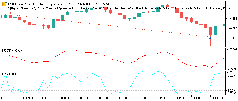
Pattern-1

The bearish signal is registered when we have negative divergence in TRIX with WPR in the resistance/overbought territory.

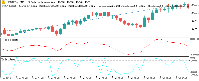
Pattern-4

Bullish signal has TRIX, breaking through a resistance while WPR is between -50 and -20.

Pattern-5

The bearish signal is when the TRIX is reversing from an oversold level with WPR exiting oversold suggesting a potential pullback to a bearish trend.

Deep Q Networks - Value Based Reinforcement Learning

In order to better appreciate why DQNs are well poised for trading use, it could be constructive to start by revisiting the fundamentals of reinforcement learning. At its core, RL is a systematic way in which an agent interacts with a given environment. On each time step or interval, this agent observes the present state, takes action, and then gets rewarded for it in proportion to the desirability of the action it has taken. The agent’s end game is to garner as much cumulative reward, over time, as possible; something it is able to achieve if its policy, the mapping of states to actions, also improves over time. 

In the markets, the state could include a collection of technical indicators, as mentioned above, that could range from raw values to pipeline transformations. Actions, also as highlighted, can point to trading decisions of going long, short, or staying neutral. The reward the agent receives, is typically expressed in terms of profit and loss with sometimes transaction costs, or even excursion exposures factored in. A point of note here though is that unlike supervised learning, there is no single correct answer to copy. Rather, the agent is tasked with discovering, primarily by exploration, which choices consistently result in more rewards.

A DQN builds on the precept of Q-Learning. This, is one of the more established value-based algorithms in reinforcement learning, and it introduces the notion of a Q-Value function. This is we represent as Q(s, a) where it is tasked with estimating the expected future reward of taking as action- a when the agent observes a state- s, and subsequently abides by the optimal policy. If this Q-function is accurate, the most suitable action at any picked moment will be the one with the highest Q-Value. Q-Learning implementations that are classic store these Q-Values in a table, which is feasible only once the action space and state dimensions are feasible.

The Financial markets, however, often produce continuous and high-dimensional states that make methods that are tabular not very practical. In this caveat is where deep learning extends this method. Rather than depending on a lookup table, a deep neural network estimates the Q-function. It is this symbiosis of reinforcement learning with deep learning that forms the genesis of the Deep-Q-Network.

The process of training a DQN does mirror the iterative as well as adaptive nature of trading itself. Transitions that consist of the state, action, reward, and then the next state, followed by a termination flag, get stored in a replay buffer. The network then gets trained on mini-batches that are randomly sampled from this buffer. This random sampling is meant to reduce the correlation between consecutive samples and therefore stabilize the learning process.

Another feature of this approach is the engagement of a target network. This network, that gets slowly updated, is a copy of the Q-Network. Its purpose is to prevent destabilizing feedback loops that are bound to happen when the network learns directly from its own constantly revised forecasts. This particular update mechanism depends on the Bellman equation, where the network parameters get some adjustment in order to minimize the difference between rewards and estimates that are discounted off the future returns. The ability to explore is kept by bringing in some randomness into the agent’s decisions. This is often in the form of an epsilon-greedy policy, whose goal is to ensure the model does not get trapped in premature exploitation of a single pattern. Epsilon is an almost zero floating value, so this is usually a very small percent.

In terms of trading, this process does imply that the network slowly gets able to learn and process which patterns of the indicators are more likely to appear before certain profitable setups. This all happens while it is still testing alternative indicator options in order to avoid overfitting to historical data or, more succinctly, the recency bias.  DQNs have a habit of excelling in this setting because they are capable of naturally fitting in discrete action spaces such as whether to go long-short-neutral. They do this while still being able to learn adaptively instead of relying on static thresholds. More importantly, though, they have the capacity to incorporate the reality of delayed rewards, given that profitability does not necessarily always materialize as soon as a decision is taken. Therefore, by discounting future rewards, the DQN tends to balance immediate payoffs against long-term profitability.

In our study for this article, the features are got from TRIX and WPR in order to determine the state input. The discrete actions are going to correspond to the trade positions open to a trader to embark on. These can encompass pending orders, if one seeks to be more elaborate, but we are going to stick to just long, short, and neutral. Training a DQN on historical data does allow the model to capture the interactions that can be between these indicators and may not be obvious when applying fixed rules. With this approach, the network gets capable of assigning relative values in proportion to actions. This has the effect of transforming raw technical indicator signals into actionable trading policies that bring together adaptability and foresight.

Value-Based RL vs Policy and Actor-Critic Methods

I thought I would also include a comparison between these two. Deep Q networks  do belong to the family of value-based reinforcement learning algorithms, that are marked by their emphasis on estimating the value of actions as opposed to learning a direct pseudo mapping from states to actions. Said differently, a value-based agent tries to get an answer to the question: “If I take this action now, how much reward in the long-term can I expect to receive”? In contrast, alternative reinforcement learning methods tend to dwell, not on valuing actions, but rather on shaping the policy directly or by balancing both valuation and policy learning in some form. Getting a grasp of these differences can be key, especially when one is considering the extent to which every method aligns with the unique requirements of trading successfully in the markets. 

Methods that are policy-based, such as the REINFORCE, or Proximal Policy Optimization (PPO), do not even estimate the Q-Values at all. Rather, they turn into parameters the-policy itself such that it becomes a probability distribution over possible actions. The process of learning therefore does adjust in order for the actions leading to higher cumulative rewards to get sampled more frequently. An approach such as this is particularly beneficial in environments where the action spaces are continuous and where discretizing every possible choice would not be feasible. For traders, policy-based methods, in principle, have the potential to generate a continuous range of positions sizes, that can even be signed (as + or -) to indicate long vs short, as opposed to being restricted to our tight space of 3: long, short, or neutral. However, policy gradient methods usually suffer from high variance when updating and this usually requires more data for stabilization when one compares this to value-based methods.

Actor-Critic approaches do try to bring together the strengths of the two worlds. When this hybrid is in play, the ‘actor’ does refer to the policy, and it gets to determine which actions to engage. The ‘critic’ on the other hand evaluates these selected actions by providing an estimate of their value. By thus having this pair of components working together, actor-critic algorithms can bring stability to the learning process  and make policy updates more efficient. Within financial markets, actor-critic approaches could enable a model to propose trading actions to a varying intensity, when at the same time the critic is engaged to refine these action choices. Well-established instance of this pairing do include Advantage Actor-Critic (A2C), Deep Deterministic Policy Gradient (DDPG) and the Twin Delayed DDPG (aka TD3, also covered recently).

The major thing that sets value-based and policy-based methods apart, therefore, can be found in the trade-off between simplicity and flexibility. DQNs that are value-based tend to be simpler to implement, especially in cases where the action space is naturally discrete. In addition, they have a tendency to converge much faster when in environments where delayed, but discrete rewards are common. This should make them more appealing for trade scenarios that can be configured as a choice between a limited number of options. While policy-based and actor-critic are powerful, on paper, they do bring into the foray some complexity. This in turn elevates the computational resource requirements and usually brings implementation difficulties in platforms such as ours, MetaTrader, where backpropagation of efficiently trained ONNX models cannot be natively handled. We will discuss this, later, below.

Python Implementation of the Quantile Network

The code responsible for underpinning the thesis for this article’s Expert Advisor does to a large extent give a solid example of how a Deep Q Network can be made adaptable to the trading context while using quantile regression. This we list as follows:

# ---------------------------- QR-DQN Core ---------------------------

class QuantileNetwork(nn.Module):
    def __init__(self, state_dim: int, action_dim: int, hidden: int = 256, num_quantiles: int = NUM_QUANTILES):
        super().__init__()
        self.num_quantiles = num_quantiles
        self.action_dim = action_dim
        self.fc1 = nn.Linear(state_dim, hidden)
        self.fc2 = nn.Linear(hidden, hidden)
        self.fc3 = nn.Linear(hidden, hidden)
        self.fc4 = nn.Linear(hidden, action_dim * num_quantiles)
        fanin_init(self.fc1.weight); nn.init.zeros_(self.fc1.bias)
        fanin_init(self.fc2.weight); nn.init.zeros_(self.fc2.bias)
        fanin_init(self.fc3.weight); nn.init.zeros_(self.fc3.bias)
        nn.init.uniform_(self.fc4.weight, -3e-3, 3e-3); nn.init.zeros_(self.fc4.bias)

    def forward(self, x):
        x = F.relu(self.fc1(x))
        x = F.relu(self.fc2(x))
        x = F.relu(self.fc3(x))
        q = self.fc4(x)  # [batch, action_dim * num_quantiles]
        # FIX: only one inferred dimension allowed — reshape explicitly
        return q.view(x.size(0), self.num_quantiles, self.action_dim)  # [batch, N, A]

    def q_values(self, x):
        q = self.forward(x)            # [batch, N, A]
        return q.mean(dim=1)           # [batch, A]

The central class on our python dealings, QuantileNetwork, is in charge of approximating the Q-function. This lies at the heart of value-based reinforcement learning. Even though a regular DQN does output a single Q-Value estimate of the Q-Value of every action, the extension of this is enabled by the quantile variant in forecasting a distribution of possible outcomes. This can specifically be pertinent to trading, where, markets uncertainty is just as vital as the mean expectation. By this being able to model the complete distribution, by engaging more than one quantile, the network becomes able to capture not just the reward that is expected but also the attendant risk, per action.

Our quantile network class is structured as a fully connected neural network of four linear layers. The first three of the four layers apply linear transformations followed by a rectified linear (ReLU) activation function. This is meant to enable the network to recognize non-linear relationships between the input states and the outputted actions. The fourth and head layer, is the output, and its dimensions are set to match those of the action dimension as well as the quantile number.

When training and performing inference, this output that is flat does get reshaped into a tensor of dimensions that are batch-sized by the quantile number. In practice, this implies that for every state inputted, the network needs to have available a set of quantile-based Q-Values for all the possible actions. When we average these quantiles, the model becomes able to recover a conventional Q-Value that, while suited in decision-making, is still able to retain the flexibility paramount in risk analysis when required.

Initialization of the weights gets done very cautiously by engaging fan-in scaling for the starting layers. Small distributions that are uniform are used for the final output layer. This form of initializing is essential in reinforcement learning, given that unstable weight distributions can have tendencies to amplify any present noise in the data. This would destabilize the training process, therefore by ensuring that our starting weight parameters have some form of balance, the Quantile Network is able to a degree, to avoid premature divergence by improving its convergence in the optimization/ backpropagation process.

The agent, we use with our DQN, orchestrates the learning process by maintaining the main quantile network together with a target network, which is simply a copy of our quantile network. This copy receives periodic updates via a soft replacement mechanism. This lagged update sees to it that the targets used in training evolve smoothly instead of erratically. In addition, the agent is also key in starting an optimizer, which for our purposes is Adam. Adam is well-placed to deal with noisy gradient updates that are a major trait in reinforcement learning. Our agent listing is as follows:

class QRDQNAgent:
    def __init__(self, state_dim: int, action_dim: int, hidden: int = 256):
        self.state_dim = state_dim
        self.action_dim = action_dim
        self.num_quantiles = NUM_QUANTILES

        self.net        = QuantileNetwork(state_dim, action_dim, hidden).to(DEVICE)
        self.target_net = QuantileNetwork(state_dim, action_dim, hidden).to(DEVICE)
        self.target_net.load_state_dict(self.net.state_dict())

        self.optimizer = optim.Adam(self.net.parameters(), lr=LR)
        self.replay_buffer = ReplayBuffer(capacity=100_000, state_dim=state_dim)

        # quantile fractions τ_i (midpoints)
        self.taus = torch.linspace(0.0 + 1.0/(2*self.num_quantiles),
                                   1.0 - 1.0/(2*self.num_quantiles),
                                   self.num_quantiles, device=DEVICE).view(1, -1)  # [1, N]

    @torch.no_grad()
    def act(self, state: torch.Tensor, epsilon: float = 0.1) -> int:
        if np.random.rand() < epsilon:
            return np.random.randint(self.action_dim)
        q_vals = self.net.q_values(state.unsqueeze(0).to(DEVICE))  # [1, A]
        return int(torch.argmax(q_vals, dim=1).item())

    def _quantile_huber_loss(self, preds: torch.Tensor, target: torch.Tensor, taus: torch.Tensor) -> torch.Tensor:
        """
        preds:  [B, N]   (predicted quantiles for chosen action)
        target: [B, N]   (target quantiles)
        taus:   [1, N]
        """
        diff = target.unsqueeze(1) - preds.unsqueeze(2)  # [B, N, N]
        huber = torch.where(diff.abs() <= KAPPA,
                            0.5 * diff.pow(2),
                            KAPPA * (diff.abs() - 0.5 * KAPPA))
        tau = taus.view(1, -1, 1)  # [1, N, 1]
        loss = (torch.abs(tau - (diff.detach() < 0).float()) * huber).mean()
        return loss

    def learn(self, batch_size: int = BATCH_SIZE):
        if self.replay_buffer.size < batch_size:
            return

        s, a, r, ns, d = self.replay_buffer.sample(batch_size)

        with torch.no_grad():
            # Double DQN selection w/ target evaluation (simple variant)
            q_next_online = self.net.q_values(ns)                  # [B, A]
            a_next = q_next_online.argmax(dim=1, keepdim=True)     # [B,1]
            q_next_all = self.target_net(ns)                       # [B, N, A]
            q_next_sel = q_next_all.gather(2, a_next.unsqueeze(1).expand(-1, self.num_quantiles, 1)).squeeze(-1)  # [B, N]
            target = r + (1.0 - d) * GAMMA * q_next_sel            # broadcast [B,1] + [B,N] -> [B,N]

        q_preds_all = self.net(s)                                  # [B, N, A]
        a_expanded  = a.view(-1, 1, 1).expand(-1, self.num_quantiles, 1)  # [B, N, 1]
        q_preds     = q_preds_all.gather(2, a_expanded).squeeze(-1)       # [B, N]

        loss = self._quantile_huber_loss(q_preds, target, self.taus)

        self.optimizer.zero_grad()
        loss.backward()
        self.optimizer.step()

        # Soft update target
        with torch.no_grad():
            for tp, sp in zip(self.target_net.parameters(), self.net.parameters()):
                tp.data.mul_(1.0 - TARGET_TAU)
                tp.data.add_(TARGET_TAU * sp.data)

    # -------------------- ONNX Export --------------------
    def export_qnet_onnx(self, path: str):
        """
        Export a wrapper that outputs mean Q-values: [1, action_dim]
        """
        class QValuesHead(nn.Module):
            def __init__(self, net: QuantileNetwork):
                super().__init__()
                self.net = net
            def forward(self, x):
                return self.net.q_values(x)

        wrapper = QValuesHead(self.net).to(DEVICE).eval()
        dummy = torch.zeros(1, self.state_dim, dtype=torch.float32, device=DEVICE)
        torch.onnx.export(
            wrapper, dummy, path,
            export_params=True, opset_version=17, do_constant_folding=True,
            input_names=["state"], output_names=["q_values"], dynamic_axes=None
        )
        return path

We also need a replay buffer implementation in order to store our state transitions. Our agent is able top sample random small batches of data from this buffer in order to help de-correlate the training data, as already argued above.

Our learning process does involve the computation of a quantile Huber Loss, a metric for the gap between the forecast quantiles and the target/ expected quantiles. This is performed while remaining robust to outliers. The familiar DQN approach is used to construct the targets, with the next action getting chosen in accordance with the online network. However, the evaluation of its value comes from the target network. The effect of this is to reduce the bias that can otherwise come-up almost always when using the same network for both selection and evaluation. Our quantile Huber Loss does apply penalties, not just for forecasts whose means are amiss, but also for deviations across the distribution gamut of possible returns. This is bound to make the model more resilient in volatile and uncertain markets.

Our listing above also do have an environment class, CustomDataEnv, whose purpose is to set hoe the agent gets to interact with data that is historic. Our environment does take as input a feature matrix that is derived from TRIX and WPR indicator patterns, as well as a target array that shows subsequent price action, after the said indicator patterns were evident. For each step, the agent gets to choose an action that does correspond to either long or short or neutral. The environment then returns the next state as well as a reward that is computed as the product of both the action and the return observed, but penalized with transaction costs whenever the action has to change. This methodology is able to shift the historical data into a sequential decision-making environment where we mimic some live trading action.

At the end, the implementation gets to give an ONNX export function. Noteworthy though is that backpropagation is not feasible in MetaTrader of the exported ONNX, which unfortunately is the sole option when using python trained models. It is intended to be used only for inference. The export, however, wraps the QuantileNetwork class into a lightweight head that gives as output mean Q-Values. This guarantees the resulting model is compact and efficient sufficiently to do evaluations for an Expert Advisor. As mentioned in past articles, this step where we need to check and be certain about sizes of input and output layers is critical in maintaining our bridge between lean well-trained models and using them on live accounts.

To wrap up here, the QuantileNetwork and its agent wrapper help demonstrate how reinforcement learning concepts can be turned into usable code. The use of quantile regression does boost adaptability by capturing reward distributions; and in tandem, the replay buffer as well as target network help insert some stability in the training process, with ONNX bringing a way for real-world integration. For us traders, therefore, these python code-listings, which are not exhaustive, do give us the important first step in moving from indicator based signals to robust, data driven decision-making.

Challenges of RL and MQL5 Integration

Even though the Python use and bridging to MQL5 does showcase how reinforcement learning can be trained on historical data, moving such models into MetaTrader in general does come with some hiccups. I hinted at these in past articles, particularly in the conclusion of the last article, where we happened to use a reinforcement learning trained model. The primary limitation is that MQL5, and any platform for that matter, does not support the backpropagation of ONNX files. They were/are meant for forward passes only, at least from the latest version(s). 

Within Python, because we have the original network code as well as the expedient tensor libraries, we are able to efficiently train and back propagate networks. MQL5’s inherent limitation at the moment is that it is designed and built for efficient, lightweight execution of trade logic and not en masse numerical computations. This implies that when we export an ONNX and have it either referenced from the sandbox or embedded in the Expert Advisor, we can only do a forward inference. The weights of the exported model, as per the last and latest ONNX versions, do not allow its weights to be updated. 

This caveat, does force us into a compromise which is simply our next best alternative or strictly speaking our only option in order to use all the training of the exported model. This compromise also points to why we only export one network model to ONNX when we are going to capitalize on reinforcement learning in MQL5, for now. In the classical reinforcement learning loop, the agent is continuously interacting with the environment, storing experiences and also adjusting its Q-Values in real time. However, in our MQL5 context, training should happen wholeheartedly offline in Python. The model is meant to learn once on historical data, and once trained its network weights, layers and biases get exported it is deployed as a static actor.

Because of this, the so-called reinforcement learning system within MetaTrader is in effect a supervised learning model. It simply  maps input features of the indicators TRIX and WPR to output values that show relative desirability of trade actions. This policy, or mapping relationship, does not adapt to new or emergent states when live trading, or even forward walking.

Another hiccup, albeit a manageable one, is in the expectation alignment of the ONNX runtime within MQL5’s interface. ONNX models are effectively constant variables in that they expect particular input and output shapes for the respective layers. These shapes are defined within python with batch dimensions and a particular floating point precision, whether 32 or 64. If the container shapes declared in MQL5, when the ONNX handles are being initialized, do not match what was set in python, the runtime initialization will fail. This is often a solvable but sticky  point nonetheless because most people who export their models do not take time to print off the actual shapes of these input and output layers.

Good news here though is besides printing off the actual shape of these layers in python, Meta Editor now offers, under its tools' menu, a neural network viewer application. Once the application is launched, in a separate window from Meta Editor, one can proceed to open the exported ONNX file and then view its detailed layout including the sizes and shapes of the input and output layers.

Supervised Learning Compromise

With a reinforcement learning model trained in python and exported to ONNX its purpose within MQL5 changes remarkably. The model can no longer, as intended and designed, it is no longer an adaptive learner but a static decision engine. In practice, this implies the exported actor network is used like any other predictive supervised learning network. It does so, having been trained as a reinforcement learning network, meaning its number of layers, layer size, and other architecture details may not be as endearing as those of equivalent supervised learning models, that are designed and trained as such. Our compromising approach nevertheless allows integration of some more logic into MQL5, which, though possible without python and ONNX, cannot be incorporated as efficiently.

So, our compromised implementation starts with embedding the actor ONNX files directly into MQL5 as resources. These ONNX files are essentially the weights, biases and layer sizes of our trained quantile network. It gets compressed into a format that MQL5 runtime can process efficiently. In our custom signal class, the three models for the patterns 1, 4, and 5 are referenced, where each one corresponds to a unique set of indicator patterns from the indicators TRIX and WPR. When initializing, the Expert Advisor creates ONNX handles from these buffers, seeing to it that all the networks can be called when evaluating conditions for trade entries. When we are here, the model is not retrained or changed, but it is simply loaded into memory as a reference tool that is ready to use.

Signal Logic

Once ONNX is exported and embedded in MQL5, one of the key steps that follows is composing the signal code and open position conditions. This is the code that translates the quantile network outputs into meaningful trade conditions. This logic that we refer to is listed in the LongCondition and ShortCondition functions within the custom signal class as follows:

//+------------------------------------------------------------------+
//| "Voting" that price will grow.                                   |
//+------------------------------------------------------------------+
int CSignalRL_TRX_WPR::LongCondition(void)
{  int result  = 0, results = 0;
   vectorf _x;
   _x.Init(2);
   _x.Fill(0.0);
//--- if the model 1 is used
   if(((m_patterns_usage & 0x02) != 0) && IsPattern_1(POSITION_TYPE_BUY))
   {  _x[0] = 1.0f;
      double _y = RunModel(0, POSITION_TYPE_BUY, _x);
      if(_y > 0.0)
      {  result += m_pattern_1;
         results++;
      }
   }
//--- if the model 4 is used
   if(((m_patterns_usage & 0x10) != 0) && IsPattern_4(POSITION_TYPE_BUY))
   {  _x[0] = 1.0f;
      double _y = RunModel(0, POSITION_TYPE_BUY, _x);
      if(_y > 0.0)
      {  result += m_pattern_4;
         results++;
      }
   }
//--- if the model 5 is used
   if(((m_patterns_usage & 0x20) != 0) && IsPattern_5(POSITION_TYPE_BUY))
   {  _x[0] = 1.0f;
      double _y = RunModel(0, POSITION_TYPE_BUY, _x);
      if(_y > 0.0)
      {  result += m_pattern_5;
         results++;
      }
   }
//--- return the result
//if(result > 0)printf(__FUNCSIG__+" result is: %i",result);
   if(results > 0 && result > 0)
   {  return(int(round(result / results)));
   }
   return(0);
}
//+------------------------------------------------------------------+
//| "Voting" that price will fall.                                   |
//+------------------------------------------------------------------+
int CSignalRL_TRX_WPR::ShortCondition(void)
{  int result  = 0, results = 0;
   vectorf _x;
   _x.Init(2);
   _x.Fill(0.0);
//--- if the model 1 is used
   if(((m_patterns_usage & 0x02) != 0) && IsPattern_1(POSITION_TYPE_SELL))
   {  _x[1] = 1.0f;
      double _y = RunModel(0, POSITION_TYPE_SELL, _x);
      if(_y < 0.0)
      {  result += m_pattern_1;
         results++;
      }
   }
//--- if the model 4 is used
   if(((m_patterns_usage & 0x10) != 0) && IsPattern_4(POSITION_TYPE_SELL))
   {  _x[1] = 1.0f;
      double _y = RunModel(0, POSITION_TYPE_SELL, _x);
      if(_y < 0.0)
      {  result += m_pattern_4;
         results++;
      }
   }
//--- if the model 5 is used
   if(((m_patterns_usage & 0x20) != 0) && IsPattern_5(POSITION_TYPE_SELL))
   {  _x[1] = 1.0f;
      double _y = RunModel(0, POSITION_TYPE_SELL, _x);
      if(_y < 0.0)
      {  result += m_pattern_5;
         results++;
      }
   }
//--- return the result
//if(result > 0)printf(__FUNCSIG__+" result is: %i",result);
   if(results > 0 && result > 0)
   {  return(int(round(result / results)));
   }
   return(0);
}

Our listing of these two methods above determine the core of how the Expert Advisor decides when to open buy or sell positions. It does so by merging the pattern recognition of technical indicators with the decision outputs of the reinforcement learning outputs.

The long function starts by declaring a feature vector that stands for the input state. This vector, x, is initialized and then filled with zeroes. Once this is done, we selectively get to assign 1 to one of its 2 indices firstly, depending on which patterns are in use by the Expert Advisor. To recap, this is the significance of the input parameter, ‘patterns-used’.

If a pattern is indexed 1, for example, then we have to set the parameter ‘Patterns-Used’ to 2 to the power 1 which comes to 2. If the index is 2 then this is 2 to the power 2 which comes to 4, and so on. The maximum value that this parameter can be assigned, meaningfully, is 1023 since we have only 10 parameters. Any number between 0 and 1023 that is not a pure exponent of 2 would represent a combination of these patterns, and the reader could explore setting up the expert Advisor to use multiple patterns. However, based on our arguments and test results presented in past articles we choose not to explore this avenue within these series, for now.

We are using only patterns 1, 4, and 5 and so those are the patterns we only have to check for. If pattern-1 conditions are met, the first index of the vector gets assigned a 1. This is also done when we are trading with pattern 4, or pattern 5. Note that even though on paper this Expert Advisor can have the input parameter patterns used adjusted to allow multiple-pattern-use as explained in the italics above, we are strictly using one pattern at a time only. In fact, multiple pattern use is bound to yield very undependable test results since cross signal cancellation will be rife.

Once an in use pattern is matched, the optimized weight as well as an ONNX forwards pass contribute to the final result of the condition. The ShortCondition also mirrors this logic but focusing on sell pattern opportunities. The x feature vector is declared, and similar pattern checks are performed. The main distinction here, keeping with logic we have always been using, is that on a pattern match that is affirmed by the quantile network, we assign the 1 to the second index, not the first. All other weighting averages and computing of the result value matches what is in the long condition.

Test Results

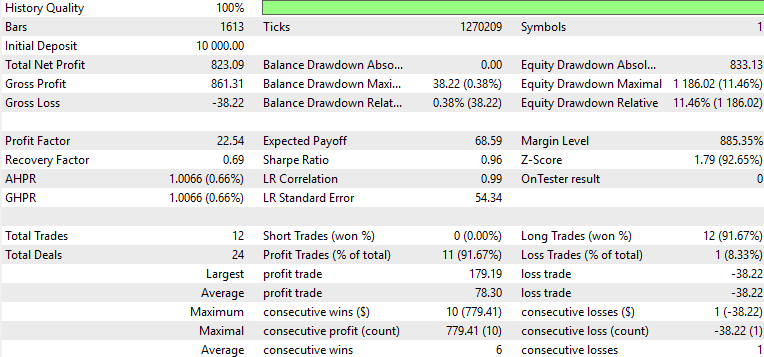
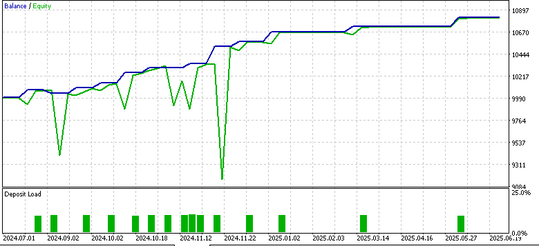
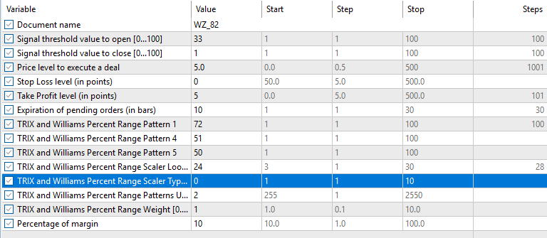
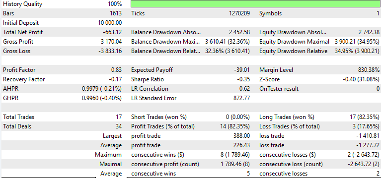
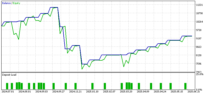
We tested the symbol EUR USD on the 4-hour time frame from 2023.07.01 to 2024.07.01 when training and optimizing. The forward walk window was from 2024.07.01 TO 2025.07.01, and this gave us the following results for the three patterns 1, 4, and 5.

Pattern-1

Pattern-4

Pattern-5

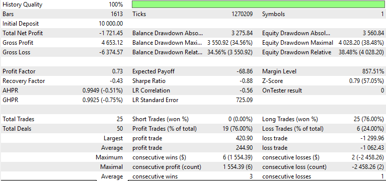
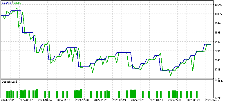
Only pattern 1 appeared to forward walk profitably, while 4 and 5 struggled. The usual caveats of this not being financial advice apply, however the use of ‘weak’/ unadapted actor networks as supervised learning models could be to blame. Our purpose here as always is never to provide out of box solutions but rather to probe from a diverse array of opportunities and attempt to exhibit what is possible. The finishing work and important deliginece is always on the part of the reader, should he choose to incorporate some of the ideas presented here.

Conclusion

Our article on the TRIX and WPR signal patterns within a reinforcement learning framework has shown both the promise and limit of MQL5 for now. Python modules get updated all the time so it could be at some point in the future the ONNX exported networks will be updatable with backpropagation abilities. For now, it is not the case so that is a limitation. Models need to be trained offline and then ‘cast in stone’, such that they operate as inference engines.

name	description
WZ_82.mq5	Wizard assembled Expert Main File whose header lists referenced files
SignalWZ_82.mqh	Custom signal class that imports DQNs
82_5_0.onnx	ONNX Exported model for pattern-5
82_4_0.onnx	ONNX Exported model for pattern-4
82_1_0.onnx	ONNX Exported model for pattern-1

Guidance on how to use the attached files can be found here for new readers.