Overcoming The Limitation of Machine Learning (Part 4): Overcoming Irreducible Error Using Multiple Forecast Horizons

MetaTrader 5 — Examples | 23 September 2025, 09:01

1 360

Machine learning is a very broad field that can be studied and interpreted from many different perspectives. This very breadth makes it materially challenging for any one of us to master. In our series of articles, we have covered some material on machine learning from a statistical point of view, or from the perspective of linear algebra. However, we rarely give attention to the geometric interpretation of machine learning models. Traditionally, machine learning models are described as approximating a function that maps inputs to outputs. From a geometric perspective, however, this is incomplete.

What models actually do is embed images of the target onto the space defined by the inputs, so that in the future they can attempt to describe the target using only those inputs. In doing so, the model defines a new manifold from the input data and makes predictions on this new manifold. But the true target lives on its own manifold. This misalignment creates a subtle but unavoidable form of irreducible error: the model is never truly pointing at the target, but rather, the model can only point at some combination of the inputs.

A thought experiment may help. Imagine you are given recordings of the speeds of two cars and asked to judge which one is faster. Easy enough — until you discover one car’s speed is measured in miles per minute and the other in kilometers per hour. Your judgments become unreliable because the measurements live in different units. Likewise, the model’s predictions are expressed in a coordinate system different from the one where the true target lives. That is to say, the model is permitted to create its own units on the fly.

Sometimes such unit mismatches are harmless, in cases where the target truly lives within the span of the inputs this misalignment error can be almost equal to 0. But in trading, ignoring them can be costly. Machine learning models perform coordinate transformations behind the scenes, placing us in a coordinate system different from the target's. In financial markets, unlike in the natural sciences, we are not guaranteed that our inputs perfectly explain the target. Here, we are working partly blind.

In our related series on self-optimizing expert advisors, we discussed how linear regression models could be constructed using matrix factorization, introduced the OpenBLAS library, and explained singular value decomposition (SVD). Readers unfamiliar with that discussion should review it, as this article builds on that foundation, a link is provided, here.

For returning readers, recall that SVD factorizes a matrix into three smaller matrices: U, S and VT. Each has special geometric properties. U and VT are orthogonal matrices, meaning they represent rotations or reflections of the original data — and crucially, they do not stretch vectors, they only change direction. S, the middle matrix, is diagonal and scales the data values.

Taken together, SVD can be understood as a sequence of rotation, scaling, and rotation applied to the data. This is how linear regression models embed images of the target onto the space of the inputs. Therefore, if we strip linear regression down to its geometric essence, it is simply rotating, scaling, and rotating again. Nothing more. That’s it. Rotate, scale, rotate. Studying geometry will teach you to see it this way, but once you do so, a provocative question emerges: where is all the “learning” truly happening?

The answer is unsettling. What practitioners call “learning” is, in fact, nothing more than aligning coordinate systems and rescaling axes so the target can be projected into the span of the inputs. We are not uncovering hidden truths in the data. We are applying a sequence of geometric transformations until two manifolds line up just enough for predictions to look reasonable.

In fact, SVD is the process by which the new coordinate system is generated. In linear regression, the input data is being projected onto a set of orthogonal axes, scaled, and rotated back, creating a transformed space in which the target can be approximated as closely as possible. The model’s “learning” is really just the alignment of the target with this new coordinate system.

From this geometric framing, we can motivate actions and domain bound best practices that would otherwise seem unfounded. The key takeaway is that we must stop making direct comparisons between the predictions of a model and the real value of the target. Instead, we should compare the model’s predictions against each other, at different horizons.

For example, suppose the model predicts that the close price one step ahead will be $5, and ten steps ahead will be $15. The slope between these forecasts is positive, so we buy. If the slope is negative, we sell. We stop expecting predictions to perfectly match reality — because manifold misalignment may forever make that impossible — and instead trade on the relative slope of the forecasts. This multi-step prediction format is not new to algorithmic trading, but rather this article is aiming to communicate to the reader that multi-step predictions should be the DeFacto gold-standard when employing machine learning models.

This article makes no claim to reduce or eliminate the geometric error. Instead, it teaches how to minimize our interaction with it, by staying outside the domain where the error dominates.

In our methodology, we began with a machine learning model trained on nine different targets. These targets were comprised of the close, high and low moving average at 1, 5 and 10 daily candles in the future. The control setup followed the classical approach: predict the real value of the target 1 candle in the future, compare it to the current value of the target, and trade accordingly. As the reader will see, we repeatedly outperformed this classical methodology by abandoning direct comparisons and instead comparing the model’s own predictions across multiple horizons. The general idea is simple but powerful: our model's predictions may be more profitable for us when compared against themselves than when compared against the real target.

We back tested the control setup on 3 years of historical data spanning from March 2022 until May 2025. The control setup produced a net profit of $71 over this period. By only changing how we interpret the model's predictions, we raised net profit to $180, a 153% improvement in profitability. Our Sharpe ratio appreciated from 0.45 to 2.16 and our percentage of profitable trades rose from 46% to 65%, this represents a 41% improvement in trading accuracy.

The key takeaway is that all the improvements we shall now demonstrate to the reader will be performed without ever swapping the model we are depending on and can be extended to any other machine learning model the reader already knows.

Fetching Market Data

We begin by writing an MQL5 script to fetch the historical market data we need. Extracting historical market data from your MetaTrader 5 terminal is best practice because it ensures that our ONNX models will be trained on historical data that is consistent with the final production environment. Our MQL5 script fetches detailed recordings on the four dominant price levels and their moving averages. We also pay attention to the growth in each of these price levels when compared to their previous levels 5 steps in the past. All this data is written out to CSV and saved on your hard drive.

//+------------------------------------------------------------------+
//|                                                      ProjectName |
//|                                      Copyright 2020, CompanyName |
//|                                       http://www.companyname.net |
//+------------------------------------------------------------------+
#property copyright "Copyright 2024, MetaQuotes Ltd."
#property link      "https://www.mql5.com"
#property version   "1.00"
#property script_show_inputs

//--- Define our moving average indicator
#define MA_PERIOD 5                 //--- Moving Average Period
#define MA_TYPE   MODE_SMA          //--- Type of moving average we have
#define HORIZON   5                 //--- Forecast horizon

//--- Our handlers for our indicators
int ma_handle,ma_o_handle,ma_h_handle,ma_l_handle;

//--- Data structures to store the readings from our indicators
double ma_reading[],ma_o_reading[],ma_h_reading[],ma_l_reading[];

//--- File name
string file_name = Symbol() + " Detailed Market Data As Series Moving Average.csv";

//--- Amount of data requested
input int size = 3000;

//+------------------------------------------------------------------+
//| Our script execution                                             |
//+------------------------------------------------------------------+
void OnStart()
  {
   int fetch = size + (HORIZON * 2);
//---Setup our technical indicators
   ma_handle = iMA(_Symbol,PERIOD_CURRENT,MA_PERIOD,0,MA_TYPE,PRICE_CLOSE);
   ma_o_handle = iMA(_Symbol,PERIOD_CURRENT,MA_PERIOD,0,MA_TYPE,PRICE_OPEN);
   ma_h_handle = iMA(_Symbol,PERIOD_CURRENT,MA_PERIOD,0,MA_TYPE,PRICE_HIGH);
   ma_l_handle = iMA(_Symbol,PERIOD_CURRENT,MA_PERIOD,0,MA_TYPE,PRICE_LOW);

//---Set the values as series
   CopyBuffer(ma_handle,0,0,fetch,ma_reading);
   ArraySetAsSeries(ma_reading,true);
   CopyBuffer(ma_o_handle,0,0,fetch,ma_o_reading);
   ArraySetAsSeries(ma_o_reading,true);
   CopyBuffer(ma_h_handle,0,0,fetch,ma_h_reading);
   ArraySetAsSeries(ma_h_reading,true);
   CopyBuffer(ma_l_handle,0,0,fetch,ma_l_reading);
   ArraySetAsSeries(ma_l_reading,true);

//---Write to file
   int file_handle=FileOpen(file_name,FILE_WRITE|FILE_ANSI|FILE_CSV,",");

   for(int i=size;i>=1;i--)
     {
      if(i == size)
        {
         FileWrite(file_handle,"Time",
                   //--- OHLC
                   "True Open",
                   "True High",
                   "True Low",
                   "True Close",
                   //--- MA OHLC
                   "True MA C",
                   "True MA O",
                   "True MA H",
                   "True MA L",
                   //--- Growth in OHLC
                   "Diff Open",
                   "Diff High",
                   "Diff Low",
                   "Diff Close",
                   //--- Growth in MA OHLC
                   "Diff MA Close 2",
                   "Diff MA Open 2",
                   "Diff MA High 2",
                   "Diff MA Low 2"
                  );
        }

      else
        {
         FileWrite(file_handle,
                   iTime(_Symbol,PERIOD_CURRENT,i),
                   //--- OHLC
                   iClose(_Symbol,PERIOD_CURRENT,i),
                   iOpen(_Symbol,PERIOD_CURRENT,i),
                   iHigh(_Symbol,PERIOD_CURRENT,i),
                   iLow(_Symbol,PERIOD_CURRENT,i),
                   //--- MA OHLC
                   ma_reading[i],
                   ma_o_reading[i],
                   ma_h_reading[i],
                   ma_l_reading[i],
                   //--- Growth in OHLC
                   iOpen(_Symbol,PERIOD_CURRENT,i)   - iOpen(_Symbol,PERIOD_CURRENT,(i + HORIZON)),
                   iHigh(_Symbol,PERIOD_CURRENT,i)   - iHigh(_Symbol,PERIOD_CURRENT,(i + HORIZON)),
                   iLow(_Symbol,PERIOD_CURRENT,i)    - iLow(_Symbol,PERIOD_CURRENT,(i + HORIZON)),
                   iClose(_Symbol,PERIOD_CURRENT,i)  - iClose(_Symbol,PERIOD_CURRENT,(i + HORIZON)),
                   //--- Growth in MA OHLC
                   ma_reading[i] - ma_reading[(i + HORIZON)],
                   ma_o_reading[i] - ma_o_reading[(i + HORIZON)],
                   ma_h_reading[i] - ma_h_reading[(i + HORIZON)],
                   ma_l_reading[i] - ma_l_reading[(i + HORIZON)]
                  );
        }
     }
//--- Close the file
   FileClose(file_handle);
  }
//+------------------------------------------------------------------+

//+------------------------------------------------------------------+
//| Undefine system constants                                        |
//+------------------------------------------------------------------+
#undef HORIZON
#undef MA_PERIOD
#undef MA_TYPE
//+------------------------------------------------------------------+

Analyzing Market Data

We can now get ready to read in our historical market data. First, load a few python libraries for data manipulation.

import pandas as pd
import numpy as np
import matplotlib.pyplot as plt

Now, we shall define 3 unique time horizons we want to forecast.

#Define our different forecast horizons
H1 = 1
H2 = 5
H3 = 10

We will now read the market data we exported from our terminal and create targets for the moving averages at different time horizons.

#Read in the data
data = pd.read_csv('../EURUSD Detailed Market Data As Series Moving Average.csv')

#Label the data
data['Target 1'] = data['True MA C'].shift(-H1)
data['Target 2'] = data['True MA C'].shift(-H2)
data['Target 3'] = data['True MA C'].shift(-H3)
data['Target 4'] = data['True MA H'].shift(-H1)
data['Target 5'] = data['True MA H'].shift(-H2)
data['Target 6'] = data['True MA H'].shift(-H3)
data['Target 7'] = data['True MA L'].shift(-H1)
data['Target 8'] = data['True MA L'].shift(-H2)
data['Target 9'] = data['True MA L'].shift(-H3)

#Drop missing rows
data = data.iloc[:-H3,:]

Create a training partition.

data      = data.iloc[:-(365*3),:]
data_test = data.iloc[-(365*3):,:]

Separate the inputs and the targets.

X = data.iloc[:,1:-9]
y = data.iloc[:,-9:]

Load any machine learning model of your choice. For our discussion we shall use the sklearn library and demonstrate the principles at hand using a linear model.

from sklearn.linear_model import LinearRegression

Initialize the model.

model = LinearRegression()

Fit the model.

model.fit(X,y)

Obtain the model's predictions on the test set, but do not fit the model on the test set. As we can see the model's predictions appear to align well with target, but as we shall now see, our model can still perform even better than this.

preds = pd.DataFrame(model.predict(data_test.iloc[:,1:-9]))
plt.plot(data_test.iloc[:,-9].reset_index(drop=True),color='black')
plt.plot(preds.iloc[:,0],color='red',linestyle=':')
plt.grid()
plt.title("Out Of Sample Forecasting")
plt.ylabel('EUR/USD Exchange Rate')
plt.xlabel('Time')
plt.legend(['Actual Price','Forecasted Price'])

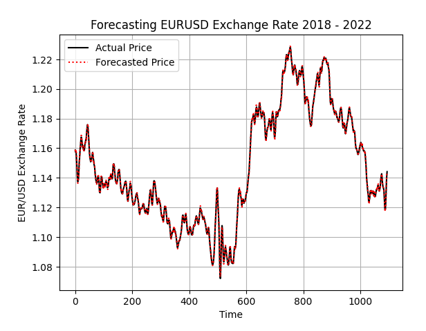
Figure 1: The model's out of sample predictions appear coherent with the real target, but this level of performance can be outperformed

ONNX stands for Open Neural Network Exchange, and it allows us to build and deploy machine learning models in a standardized library that is being adopted by an ever-growing number of programming languages. We will use the ONNX library to export our machine learning model from Python, and then subsequently import it into MQL5. ONNX allows us to rapidly develop machine learning models and deploy them.

import onnx
from skl2onnx import convert_sklearn
from skl2onnx.common.data_types import FloatTensorType

We must define the input and output shape of our ONNX models. This can be easily done because we separated inputs and outputs earlier. Simply fetch the number of columns in each partition and store them. Pandas makes this information trivial to fetch by using the shape property.

initial_types = [("FLOAT INPUT",FloatTensorType([1,X.shape[1]]))]
final_types = [("FLOAT OUTPUT",FloatTensorType([y.shape[1],1]))]

Create an ONNX prototype of the machine learning model. We shall specify the number of inputs and outputs that we need for our model.

model_proto = convert_sklearn(model,initial_types=initial_types,target_opset=12)

Save the ONNX model to disk.

onnx.save(model_proto,"EURUSD MFH LR D1.onnx")

Establishing A Baseline Performance Level

We are now ready to establish a baseline level of performance. We begin by fixing as many parameters of the strategy as possible, to ensure consistent tests.

//+------------------------------------------------------------------+
//|                                                          MFH.mq5 |
//|                                               Gamuchirai Ndawana |
//|                    https://www.mql5.com/en/users/gamuchiraindawa |
//+------------------------------------------------------------------+
#property copyright "Gamuchirai Ndawana"
#property link      "https://www.mql5.com/en/users/gamuchiraindawa"
#property version   "1.00"

//+------------------------------------------------------------------+
//| System definitions                                               |
//+------------------------------------------------------------------+
#define SYSTEM_INPUTS  16
#define SYSTEM_OUTPUTS 9
#define ATR_PERIOD     14
#define ATR_PADDING    1
#define TF_1           PERIOD_D1
#define TF_2           PERIOD_M15
#define MA_PERIOD      5
#define MA_TYPE        MODE_SMA
#define HORIZON        5

Load the ONNX buffer we exported from Python.

//+------------------------------------------------------------------+
//| System resources                                                 |
//+------------------------------------------------------------------+
#resource "\\Files\\EURUSD MFH LR D1.onnx" as const uchar onnx_buffer[];

We shall also depend on a few libraries to handle routine tasks for our algorithmic trading, such as trade execution, candle formation and handling the ONNX buffer.

//+------------------------------------------------------------------+
//| System libraries                                                 |
//+------------------------------------------------------------------+
#include <Trade\Trade.mqh>
#include <VolatilityDoctor\ONNX\ONNXFloat.mqh>
#include <VolatilityDoctor\Time\Time.mqh>
#include <VolatilityDoctor\Trade\TradeInfo.mqh>

ONNXFloat      *ONNXHandler;
Time           *TimeHandler;
Time           *LowerTimeHandler;
TradeInfo      *TradeHandler;
CTrade         Trade;

A handful of global variables are necessary, mainly for handling the technical indicators and storing the ONNX model's predictions.

//+------------------------------------------------------------------+
//| Global variables                                                 |
//+------------------------------------------------------------------+
int ma_handle,ma_o_handle,ma_h_handle,ma_l_handle,fetch,atr_handler;
double ma_reading[],ma_o_reading[],ma_h_reading[],ma_l_reading[],atr[];
double padding;
vector model_prediction;

When our application is first loaded, we shall initialize our global variables and custom classes and also store handlers to the technical indicators we created.

//+------------------------------------------------------------------+
//| Expert initialization function                                   |
//+------------------------------------------------------------------+
int OnInit()
  {
//---
   fetch            = HORIZON * 2;
   ONNXHandler      = new ONNXFloat(onnx_buffer);
   LowerTimeHandler = new Time(Symbol(),TF_2);
   TimeHandler      = new Time(Symbol(),TF_1);
   TradeHandler     = new TradeInfo(Symbol(),TF_1);

   ONNXHandler.DefineOnnxInputShape(0,1,SYSTEM_INPUTS);
   ONNXHandler.DefineOnnxOutputShape(0,1,SYSTEM_OUTPUTS);

   ma_handle        = iMA(Symbol(),TF_1,MA_PERIOD,0,MA_TYPE,PRICE_CLOSE);
   ma_o_handle      = iMA(Symbol(),TF_1,MA_PERIOD,0,MA_TYPE,PRICE_OPEN);
   ma_h_handle      = iMA(Symbol(),TF_1,MA_PERIOD,0,MA_TYPE,PRICE_HIGH);
   ma_l_handle      = iMA(Symbol(),TF_1,MA_PERIOD,0,MA_TYPE,PRICE_LOW);
   atr_handler      = iATR(Symbol(),TF_1,MA_PERIOD);

   model_prediction = vector::Zeros(SYSTEM_OUTPUTS);
//---
   return(INIT_SUCCEEDED);
  }

It is standard practice in MQL5 to practice good memory management and free up resources you are no longer using.

//+------------------------------------------------------------------+
//| Expert deinitialization function                                 |
//+------------------------------------------------------------------+
void OnDeinit(const int reason)
  {
//---
   delete ONNXHandler;
   IndicatorRelease(ma_h_handle);
   IndicatorRelease(ma_o_handle);
   IndicatorRelease(ma_l_handle);
   IndicatorRelease(ma_handle);
   IndicatorRelease(atr_handler);
  }

When new price levels have been received, we will update our technical indicator buffers and stop loss levels. Afterward, we will check if we have any open positions. If none are open, we will check for a trading opportunity, otherwise, we will manage the open position using a trailing stop loss.

//+------------------------------------------------------------------+
//| Expert tick function                                             |
//+------------------------------------------------------------------+
void OnTick()
  {
//--- Has a new candle formed
   if(TimeHandler.NewCandle())
     {
      //---Set the values as series
      CopyBuffer(ma_handle,0,0,fetch,ma_reading);
      ArraySetAsSeries(ma_reading,true);
      CopyBuffer(ma_o_handle,0,0,fetch,ma_o_reading);
      ArraySetAsSeries(ma_o_reading,true);
      CopyBuffer(ma_h_handle,0,0,fetch,ma_h_reading);
      ArraySetAsSeries(ma_h_reading,true);
      CopyBuffer(ma_l_handle,0,0,fetch,ma_l_reading);
      ArraySetAsSeries(ma_l_reading,true);
      CopyBuffer(atr_handler,0,0,fetch,atr);
      ArraySetAsSeries(atr,true);
      padding = (atr[0] * ATR_PADDING);

      //--- Obtain a prediction from our model
      if(PositionsTotal() == 0)
        {
         model_predict();
        }

      //--- Manage open positions
      if(PositionsTotal() >0)
        {
         manage_setup();
        }
     }
  }
//+------------------------------------------------------------------+

Our trailing stop loss will be defined by the ATR (Average True Range) indicator. The ATR measures market volatility and helps us dynamically adjust our risk levels. If the stop loss can be safely updated to a more profitable position, we will do so, otherwise we will wait.

//+------------------------------------------------------------------+
//| Manage our open positions                                        |
//+------------------------------------------------------------------+
void manage_setup(void)
  {
//--- Select the position by its ticket number
   if(PositionSelectByTicket(PositionGetTicket(0)))
     {
      //--- Store the current tp and sl levels
      double current_tp,current_sl;

      current_tp = PositionGetDouble(POSITION_TP);
      current_sl = PositionGetDouble(POSITION_SL);

      //--- Before we calculate the new stop loss or take profit
      double new_sl,new_tp;

      //--- We first check the position type
      if(PositionGetInteger(POSITION_TYPE) == POSITION_TYPE_BUY)
        {
         new_sl = TradeHandler.GetBid()-padding;
         new_tp = TradeHandler.GetBid()+padding;

         //--- Check if the new stops are more profitable
         if(new_sl>current_sl)
            Trade.PositionModify(Symbol(),new_sl,new_tp);
        }

      if(PositionGetInteger(POSITION_TYPE) == POSITION_TYPE_SELL)
        {
         new_sl = TradeHandler.GetAsk()+padding;
         new_tp = TradeHandler.GetAsk()-padding;

         //--- Check if the new stops are more profitable
         if(new_sl<current_sl)
            Trade.PositionModify(Symbol(),new_sl,new_tp);
        }
     }
  }

We will first test our application without a machine learning model to establish a baseline level of profitability. We will use a simple break out strategy for our machine learning models to outperform. Models that fall beneath this level of performance are unacceptable.

//+------------------------------------------------------------------+
//| Obtain a prediction from our model                               |
//+------------------------------------------------------------------+
void model_predict(void)
  {
   if(iHigh(Symbol(),TF_2,1)<iOpen(Symbol(),TF_2,0))
     {
      Trade.Buy(TradeHandler.MinVolume(),TradeHandler.GetSymbol(),TradeHandler.GetAsk(),TradeHandler.GetBid()-padding,TradeHandler.GetBid()+padding);
     }


   if(iLow(Symbol(),TF_2,1)>iOpen(Symbol(),TF_2,0))
     {
      Trade.Sell(TradeHandler.MinVolume(),TradeHandler.GetSymbol(),TradeHandler.GetBid(),TradeHandler.GetAsk()+padding,TradeHandler.GetAsk()-padding);
     }
  }
//+------------------------------------------------------------------+

Lastly, undefine all system constants we created earlier.

//+------------------------------------------------------------------+
//| Undefine system constants                                        |
//+------------------------------------------------------------------+
#undef MA_PERIOD
#undef MA_TYPE
#undef HORIZON
#undef TF_1
#undef TF_2
#undef SYSTEM_INPUTS
#undef SYSTEM_OUTPUTS
#undef ATR_PADDING
#undef ATR_PERIOD

All together this is what our system looks like.

//+------------------------------------------------------------------+
//|                                                          MFH.mq5 |
//|                                               Gamuchirai Ndawana |
//|                    https://www.mql5.com/en/users/gamuchiraindawa |
//+------------------------------------------------------------------+
#property copyright "Gamuchirai Ndawana"
#property link      "https://www.mql5.com/en/users/gamuchiraindawa"
#property version   "1.00"

//+------------------------------------------------------------------+
//| System definitions                                               |
//+------------------------------------------------------------------+
#define SYSTEM_INPUTS  16
#define SYSTEM_OUTPUTS 9
#define ATR_PERIOD     14
#define ATR_PADDING    1
#define TF_1           PERIOD_D1
#define TF_2           PERIOD_M15
#define MA_PERIOD      5
#define MA_TYPE        MODE_SMA
#define HORIZON        5

//+------------------------------------------------------------------+
//| System resources                                                 |
//+------------------------------------------------------------------+
#resource "\\Files\\EURUSD MFH LR D1.onnx" as const uchar onnx_buffer[];

//+------------------------------------------------------------------+
//| System libraries                                                 |
//+------------------------------------------------------------------+
#include <Trade\Trade.mqh>
#include <VolatilityDoctor\ONNX\ONNXFloat.mqh>
#include <VolatilityDoctor\Time\Time.mqh>
#include <VolatilityDoctor\Trade\TradeInfo.mqh>

ONNXFloat      *ONNXHandler;
Time           *TimeHandler;
Time           *LowerTimeHandler;
TradeInfo      *TradeHandler;
CTrade         Trade;

//+------------------------------------------------------------------+
//| Global variables                                                 |
//+------------------------------------------------------------------+
int ma_handle,ma_o_handle,ma_h_handle,ma_l_handle,fetch,atr_handler;
double ma_reading[],ma_o_reading[],ma_h_reading[],ma_l_reading[],atr[];
double padding;
vector model_prediction;

//+------------------------------------------------------------------+
//| Expert initialization function                                   |
//+------------------------------------------------------------------+
int OnInit()
  {
//---
   fetch            = HORIZON * 2;
   ONNXHandler      = new ONNXFloat(onnx_buffer);
   LowerTimeHandler = new Time(Symbol(),TF_2);
   TimeHandler      = new Time(Symbol(),TF_1);
   TradeHandler     = new TradeInfo(Symbol(),TF_1);

   ONNXHandler.DefineOnnxInputShape(0,1,SYSTEM_INPUTS);
   ONNXHandler.DefineOnnxOutputShape(0,1,SYSTEM_OUTPUTS);

   ma_handle        = iMA(Symbol(),TF_1,MA_PERIOD,0,MA_TYPE,PRICE_CLOSE);
   ma_o_handle      = iMA(Symbol(),TF_1,MA_PERIOD,0,MA_TYPE,PRICE_OPEN);
   ma_h_handle      = iMA(Symbol(),TF_1,MA_PERIOD,0,MA_TYPE,PRICE_HIGH);
   ma_l_handle      = iMA(Symbol(),TF_1,MA_PERIOD,0,MA_TYPE,PRICE_LOW);
   atr_handler      = iATR(Symbol(),TF_1,MA_PERIOD);

   model_prediction = vector::Zeros(SYSTEM_OUTPUTS);
//---
   return(INIT_SUCCEEDED);
  }

//+------------------------------------------------------------------+
//| Expert deinitialization function                                 |
//+------------------------------------------------------------------+
void OnDeinit(const int reason)
  {
//---
   delete ONNXHandler;
   IndicatorRelease(ma_h_handle);
   IndicatorRelease(ma_o_handle);
   IndicatorRelease(ma_l_handle);
   IndicatorRelease(ma_handle);
   IndicatorRelease(atr_handler);
  }

//+------------------------------------------------------------------+
//| Expert tick function                                             |
//+------------------------------------------------------------------+
void OnTick()
  {
//--- Has a new candle formed
   if(TimeHandler.NewCandle())
     {
      //---Set the values as series
      CopyBuffer(ma_handle,0,0,fetch,ma_reading);
      ArraySetAsSeries(ma_reading,true);
      CopyBuffer(ma_o_handle,0,0,fetch,ma_o_reading);
      ArraySetAsSeries(ma_o_reading,true);
      CopyBuffer(ma_h_handle,0,0,fetch,ma_h_reading);
      ArraySetAsSeries(ma_h_reading,true);
      CopyBuffer(ma_l_handle,0,0,fetch,ma_l_reading);
      ArraySetAsSeries(ma_l_reading,true);
      CopyBuffer(atr_handler,0,0,fetch,atr);
      ArraySetAsSeries(atr,true);
      padding = (atr[0] * ATR_PADDING);
     }

   if(LowerTimeHandler.NewCandle())
     {
      //--- Obtain a prediction from our model
      if(PositionsTotal() == 0)
        {
         model_predict();
        }

      //--- Manage open positions
      if(PositionsTotal() >0)
        {
         manage_setup();
        }
     }
  }
//+------------------------------------------------------------------+

//+------------------------------------------------------------------+
//| Manage our open positions                                        |
//+------------------------------------------------------------------+
void manage_setup(void)
  {
//--- Select the position by its ticket number
   if(PositionSelectByTicket(PositionGetTicket(0)))
     {
      //--- Store the current tp and sl levels
      double current_tp,current_sl;

      current_tp = PositionGetDouble(POSITION_TP);
      current_sl = PositionGetDouble(POSITION_SL);

      //--- Before we calculate the new stop loss or take profit
      double new_sl,new_tp;

      //--- We first check the position type
      if(PositionGetInteger(POSITION_TYPE) == POSITION_TYPE_BUY)
        {
         new_sl = TradeHandler.GetBid()-padding;
         new_tp = TradeHandler.GetBid()+padding;

         //--- Check if the new stops are more profitable
         if(new_sl>current_sl)
            Trade.PositionModify(Symbol(),new_sl,new_tp);
        }

      if(PositionGetInteger(POSITION_TYPE) == POSITION_TYPE_SELL)
        {
         new_sl = TradeHandler.GetAsk()+padding;
         new_tp = TradeHandler.GetAsk()-padding;

         //--- Check if the new stops are more profitable
         if(new_sl<current_sl)
            Trade.PositionModify(Symbol(),new_sl,new_tp);
        }
     }
  }

//+------------------------------------------------------------------+
//| Obtain a prediction from our model                               |
//+------------------------------------------------------------------+
void model_predict(void)
  {
   if(iHigh(Symbol(),TF_2,1)<iOpen(Symbol(),TF_2,0))
     {
      Trade.Buy(TradeHandler.MinVolume(),TradeHandler.GetSymbol(),TradeHandler.GetAsk(),TradeHandler.GetBid()-padding,TradeHandler.GetBid()+padding);
     }


   if(iLow(Symbol(),TF_2,1)>iOpen(Symbol(),TF_2,0))
     {
      Trade.Sell(TradeHandler.MinVolume(),TradeHandler.GetSymbol(),TradeHandler.GetBid(),TradeHandler.GetAsk()+padding,TradeHandler.GetAsk()-padding);
     }
  }
//+------------------------------------------------------------------+

//+------------------------------------------------------------------+
//| Undefine system constants                                        |
//+------------------------------------------------------------------+
#undef MA_PERIOD
#undef MA_TYPE
#undef HORIZON
#undef TF_1
#undef TF_2
#undef SYSTEM_INPUTS
#undef SYSTEM_OUTPUTS
#undef ATR_PADDING
#undef ATR_PERIOD
//+------------------------------------------------------------------+

We begin by first establishing a reasonable expectation on profitability. It is materially significant to perform this step to ensure we make fair judgements on the improvements our machine learning models are truly contributing.

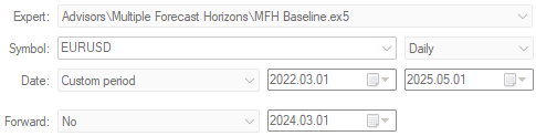
Figure 2: Selecting the back test days for our control setup

The detailed results of the control setup are given to the reader below. As we can see, majority of the trades placed by the strategy were unprofitable, however, the average profitable trade was larger than the average losing trade. This asymmetric return structure gave us confidence in the control setup.

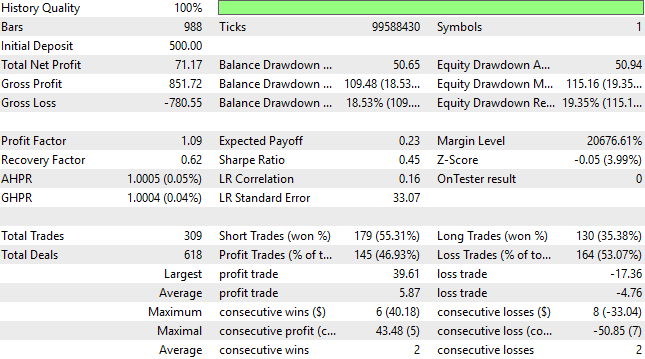
Figure 3: Analyzing the profitability of the control trading algorithm

The equity curve produced by the trading strategy, on the other hand, appears extremely volatile and gives us little confidence to continue following this trading strategy in future. Therefore, we will now attempt to employ machine learning models to iron out the volatile fluctuations in our presently simple trading strategy.

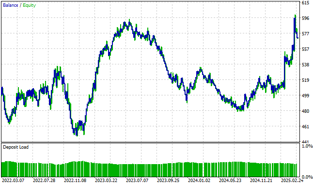
Figure 4: The original version of our trading strategy fosters little confidence in any developer

Classical Attempt To Surpass The Control

We shall now attempt to outperform the control trading strategy using the classical trading setup. Normally, in the classical setting, we forecast the target, 1 candle into the future and then compare the forecasted price against the real value of price to obtain our trading signals. This article tries to persuade the reader that this practice may not be the best possible practice for our community, let us see why.

Most of the application's code will not be changed deliberately, therefore, we can exclusively focus on the portion of MQL5 code that must be changed to test our ideas. As the reader can see below, we must now fetch the 16 inputs necessary for our ONNX model to make predictions and be sure to convert each of them to float datatypes before attempting any calculations. Afterward, we will then obtain a prediction from our ONNX model, and compare it to the real value of the target.

//+------------------------------------------------------------------+
//| Obtain a prediction from our model                               |
//+------------------------------------------------------------------+
void model_predict(void)
  {
   vectorf model_inputs(SYSTEM_INPUTS);

   model_inputs[0] = (float) iClose(_Symbol,PERIOD_CURRENT,0);
   model_inputs[1] = (float) iOpen(_Symbol,PERIOD_CURRENT,0);
   model_inputs[2] = (float) iHigh(_Symbol,PERIOD_CURRENT,0);
   model_inputs[3] = (float) iLow(_Symbol,PERIOD_CURRENT,0);
   model_inputs[4] = (float) ma_reading[0];
   model_inputs[5] = (float) ma_o_reading[0];
   model_inputs[6] = (float) ma_h_reading[0];
   model_inputs[7] = (float) ma_l_reading[0];
   model_inputs[8] = (float)(iOpen(_Symbol,PERIOD_CURRENT,0) - iOpen(_Symbol,PERIOD_CURRENT,(0 + HORIZON)));
   model_inputs[9] = (float)(iHigh(_Symbol,PERIOD_CURRENT,0)   - iHigh(_Symbol,PERIOD_CURRENT,(0 + HORIZON)));
   model_inputs[10] = (float)(iLow(_Symbol,PERIOD_CURRENT,0)    - iLow(_Symbol,PERIOD_CURRENT,(0 + HORIZON)));
   model_inputs[11] = (float)(iClose(_Symbol,PERIOD_CURRENT,0)  - iClose(_Symbol,PERIOD_CURRENT,(0 + HORIZON)));
   model_inputs[12] = (float)(ma_reading[0] - ma_reading[(0 + HORIZON)]);
   model_inputs[13] = (float)(ma_o_reading[0] - ma_o_reading[(0 + HORIZON)]);
   model_inputs[14] = (float)(ma_h_reading[0] - ma_h_reading[(0 + HORIZON)]);
   model_inputs[15] = (float)(ma_l_reading[0] - ma_l_reading[(0 + HORIZON)]);

//--- Obtain the prediction
   ONNXHandler.Predict(model_inputs);

   for(int i=0;i<SYSTEM_OUTPUTS;i++)
     {
      model_prediction[i] = ONNXHandler.GetPrediction(i);
     }

   if(iHigh(Symbol(),TF_2,1)<iOpen(Symbol(),TF_2,0))
     {
      if(model_prediction[0]>iClose(Symbol(),TF_2,0))
      Trade.Buy(TradeHandler.MinVolume(),TradeHandler.GetSymbol(),TradeHandler.GetAsk(),TradeHandler.GetBid()-padding,TradeHandler.GetBid()+padding);
     }


   if(iLow(Symbol(),TF_2,1)>iOpen(Symbol(),TF_2,0))
     {
      if(model_prediction[0]<iClose(Symbol(),TF_2,0)
      Trade.Sell(TradeHandler.MinVolume(),TradeHandler.GetSymbol(),TradeHandler.GetBid(),TradeHandler.GetAsk()+padding,TradeHandler.GetAsk()-padding);
     }
  }
//+------------------------------------------------------------------+

Running the classical machine learning trading algorithm over the same testing period we used to establish our control profitability levels.

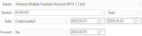
Figure 5: Performing the first attempt to outperform the control setup

The profitability levels of our trading application have depreciated dismally. Although the strategy demonstrated high accuracy with 63% of all the trades it placed being profitable, this is hardly impressive because it failed it outperform the $71 profit level established the control application.

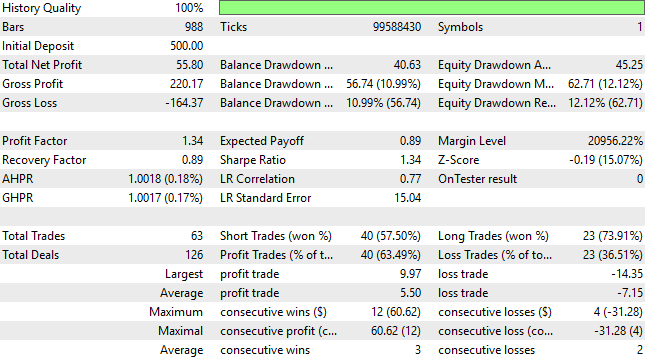
Figure 6: A detailed analysis of our first attempt to outperform the control application

The revised application we have built fails to reach the same heights as the original version of the trading strategy. But in all fairness, it is also worth noting that this version of our application also appears to be far less volatile and more reliable than the original strategy.

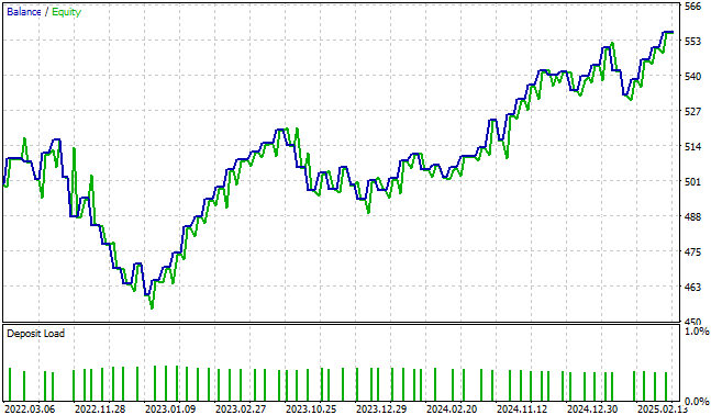
Figure 7: The equity curve produced by the improved version of our trading application is less volatile than the original strategy, but it also fails to reach the same heights

Taking The Classical Attempt To Its Limits

Recall that we are forecasting the target at 1, 5 and 10 candles into the future. Let us see if the prediction looking forward 10 candles may be more informative than the simple 1 step prediction we started with. Therefore, as we did before, we will only focus on the parts of the trading application that needed to be changed for us to make this comparison fairly.

   if(iHigh(Symbol(),TF_2,1)<iOpen(Symbol(),TF_2,0))
     {
      if(model_prediction[
    2 ]>iClose(Symbol(),TF_2,0))
         Trade.Buy(TradeHandler.MinVolume()*2,TradeHandler.GetSymbol(),TradeHandler.GetAsk(),TradeHandler.GetBid()-padding,TradeHandler.GetBid()+padding);

      Trade.Buy(TradeHandler.MinVolume(),TradeHandler.GetSymbol(),TradeHandler.GetAsk(),TradeHandler.GetBid()-padding,TradeHandler.GetBid()+padding);
     }

   if(iLow(Symbol(),TF_2,1)>iOpen(Symbol(),TF_2,0))
     {
     
      if(model_prediction[
    2 ]<iClose(Symbol(),TF_2,0))
         Trade.Sell(TradeHandler.MinVolume()*2,TradeHandler.GetSymbol(),TradeHandler.GetBid(),TradeHandler.GetAsk()+padding,TradeHandler.GetAsk()-padding);
         
      Trade.Sell(TradeHandler.MinVolume(),TradeHandler.GetSymbol(),TradeHandler.GetBid(),TradeHandler.GetAsk()+padding,TradeHandler.GetAsk()-padding);
     }

As with the control setup of the trading application, we will select the same 3-year window to test our application over.

Figure 8: Recall that all back tests must be performed over the same time period to ensure that the strategy is truly making better use of time

In most books that teach practitioners how to forecast financial markets using machine learning, forecasting 1 step into the future is commonly taught as a standard practice. However, profitable human traders rarely ever attempt to trade 1 candle at a time, and likewise as we are demonstrating in this article, our models also appear to be more profitable when permitted to look beyond the immediate candle. In fact, the reader should note, this is our first time outperforming the control setup in this discussion.

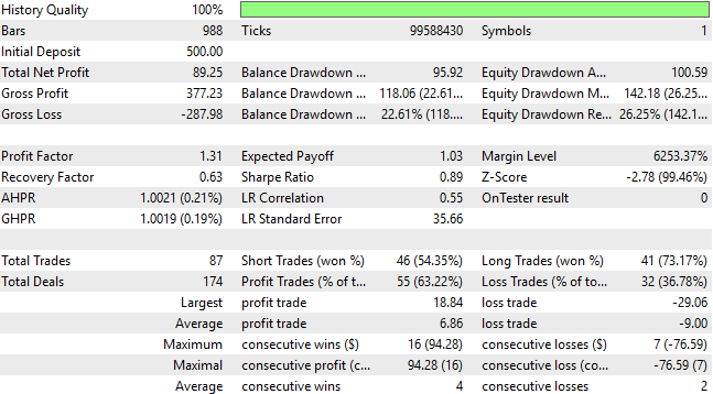
Figure 9: Forecasting 10 steps into the future appeared more profitable for us than simply forecasting 1 step into the future

Needless to say, the undesirable volatile nature of our equity curve has been corrected. This is definitely encouraging to observe, but as the reader shall soon see, we can still perform better than this.

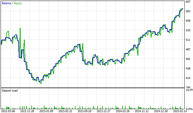
Figure 10: The equity curve produced by the second iteration of our trading application is superior to the control setup, but we shall now demonstrate to the reader how to take this to new heights

New Room For Improvement

We are now ready to compare our model's predictions at multiple time steps into the future. We will compare where the model expects the high price to be 1 and 10 steps from now, and then use the expected growth in this price level, as our trading signal.

if(iHigh(Symbol(),TF_2,1)<iOpen(Symbol(),TF_2,0))
     {
      if(model_prediction[3]<model_prediction[5])
         Trade.Buy(TradeHandler.MinVolume()*2,TradeHandler.GetSymbol(),TradeHandler.GetAsk(),TradeHandler.GetBid()-padding,TradeHandler.GetBid()+padding);

      Trade.Buy(TradeHandler.MinVolume(),TradeHandler.GetSymbol(),TradeHandler.GetAsk(),TradeHandler.GetBid()-padding,TradeHandler.GetBid()+padding);
     }

if(iLow(Symbol(),TF_2,1)>iOpen(Symbol(),TF_2,0))
     {
      if(model_prediction[3]>model_prediction[5])
         Trade.Sell(TradeHandler.MinVolume()*2,TradeHandler.GetSymbol(),TradeHandler.GetBid(),TradeHandler.GetAsk()+padding,TradeHandler.GetAsk()-padding);
         
      Trade.Sell(TradeHandler.MinVolume(),TradeHandler.GetSymbol(),TradeHandler.GetBid(),TradeHandler.GetAsk()+padding,TradeHandler.GetAsk()-padding);
     }

Let us observe if there is any merit in comparing the model's predictions over multiple time horizons, when compared with simpler direct comparisons between the model's predictions, and the real value of the target.

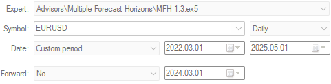
Figure 11: Running the third version of our trading application over the three-year back test period

As the reader can see, the results we have produced almost speak for themselves. Our application is now more profitable than it has ever been at any previous point in our development cycle. Recall, we are using the same ONNX model we exported earlier. And that, the root of our trading conditions has not changed. Rather, by carefully interpreting our model's predictions, we seem to be extracting more alpha from the same trading strategy.

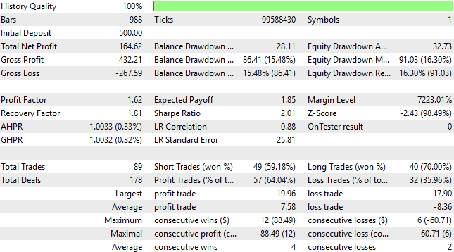
Figure 12: The detailed statistics produced by the third version of our trading application give us confidence that we have sound changes to the application

Our equity curve is consistently rising to new highs, extending far beyond the range of the control setup of our trading application or any of the profitability levels we were able to establish using the classical approach to financial machine learning.

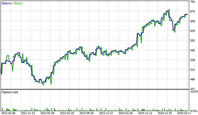
Figure 13: The equity curve produced by the current iteration of our trading application is breaking to new highs we could not reach in all the prior versions of the application.

Final Improvements

As the writer, I enjoy searching for any market structure that is easier to predict than price itself, but just as informative as knowing the future price levels themselves. Therefore, given we are dealing with moving averages on the high and low-price channel, my intuition led me to question if the growth in the midpoint between these 2 moving averages could be easier to forecast. This definitely appeared to be the case for this discussion.

if(iHigh(Symbol(),TF_2,1)<iOpen(Symbol(),TF_2,0))
     {
      if(((model_prediction[3]+model_prediction[6])/2)<((model_prediction[5]+model_prediction[8])/2))
         Trade.Buy(TradeHandler.MinVolume()*2,TradeHandler.GetSymbol(),TradeHandler.GetAsk(),TradeHandler.GetBid()-padding,TradeHandler.GetBid()+padding);

      Trade.Buy(TradeHandler.MinVolume(),TradeHandler.GetSymbol(),TradeHandler.GetAsk(),TradeHandler.GetBid()-padding,TradeHandler.GetBid()+padding);
     }

if(iLow(Symbol(),TF_2,1)>iOpen(Symbol(),TF_2,0))
     {
     
      if(((model_prediction[3]+model_prediction[6])/2)>((model_prediction[5]+model_prediction[8])/2))
         Trade.Sell(TradeHandler.MinVolume()*2,TradeHandler.GetSymbol(),TradeHandler.GetBid(),TradeHandler.GetAsk()+padding,TradeHandler.GetAsk()-padding);
         
      Trade.Sell(TradeHandler.MinVolume(),TradeHandler.GetSymbol(),TradeHandler.GetBid(),TradeHandler.GetAsk()+padding,TradeHandler.GetAsk()-padding);
     }

Run the final version of our application over the same 3-year window we have been working with.

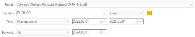
Figure 14: Running the final version of our trading application to try to outperform all the previous iterations we have built thus far

As we can see below, our application has consistently been reaching new performance levels that were out of reach for us when we began this discussion. It appears that the final version of the application we have produced so far, was worth all the effort to took to create in the first place.

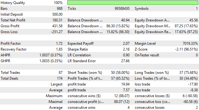
Figure 15: The final detailed performance levels of our application are superior to all other performance levels we established prior in our conversation

The volatility we observed in our equity curve is almost completely under our control. It can be remarkable how much profit can be realized, without adding any new complexity to your machine learning trading strategies.

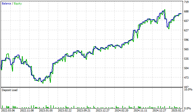
Figure 16: Visualizing the equity curve produced by the final version of our trading application gives us confidence in all the changes we have made this far

Conclusion

The idea of multiple time-step predictions is not new to the algorithmic trading community. What is new — and what this article insists upon — is the perspective that multiple time-step predictions should not be seen as an alternative technique, but rather as a candidate gold standard for algorithmic trading itself.

Earlier, I posed a question to you, the reader. I demonstrated that, from a geometric perspective, linear regression reduces to nothing more than a sequence of rotations and scalings. Then I asked: where is the learning truly happening?

For readers who still recall this question, I must offer one possible hypothesis — though I strongly prefer that you remain independent to discover your own.

The principle demonstrated throughout this article is that mathematical concepts always have geometric analogs. Every machine learning model you can think of can be reinterpreted as a coordinated acrobatics of scaling, reflection, projection, convolution, and rotation, applied to the manifolds defined by data itself. Even advanced neural networks are not mysterious: they are simply elaborate choreographies of geometric transformations, folding and reshaping data again and again.

Therefore, the answer to the question “Where is the learning happening?” may be this: learning occurs when information is encoded into geometric patterns. The cycle of rotation and scaling is one of the most elementary of these patterns. It is a powerful geometric structure, in the same sense that the three primary colors are the foundation from which all other colors are made. In geometry, there exist primary transformations from which all others are composed.

The image-classification community has already embraced this reality. Their success stems from long and detailed preprocessing pipelines — pipelines that are, in essence, a careful orchestration of geometric transformations. They may appear as routine feature engineering, but in truth, they are the quiet application of these very principles, often without full recognition of their deeper implications.

And so the reader walks away with valuable insight: multi-step forecasting in trading may be one of the most undervalued strategies in our field, precisely because it performs far more work than it is truly given credit for. Mutli-step predictions ensure we keep our comparisons in the same coordinate system. Otherwise, comparing your model's predictions directly against the real value of the target, is identical to comparing 2 quantities that aren't guaranteed to be in the same units.

File Name	File Description
Fetch_Data_MA_2.1.mq5	The MQL5 script we used to fetch historical data from our MetaTrader 5 terminal.
MFH_Baseline.mq5	The Baseline version of our trading strategy that employed no machine learning models.
MFH_1.1.mq5	The first attempt we made to build a trading application only following the classical financial machine learning paradigms.
MFH_1.2.mq5	The final attempt we made to build a trading application using the classical financial machine learning paradigms.
MFH_1.3.mq5	The first attempt we made to desist from making direct comparisons between the current price and the forecasted price.
MFH_1.4.mq5	The final version of our trading strategy that produced the highest profitability levels we demonstrated in this article.
Multiple_Forecast_Horizons.ipynb	The Jupyter Notebook we employed to export our ONNX model.

Attached files |

Download ZIP

Multiple_Forecast_Horizons.ipynb (233.21 KB)

Fetch_Data_MA_2.1.mq5 (4.79 KB)

MFH_Baseline.mq5 (7.4 KB)

MFH_1.1.mq5 (8.85 KB)

MFH_1.2.mq5 (9.17 KB)

MFH_1.3.mq5 (9.17 KB)

MFH_1.4.mq5 (9.27 KB)

Warning: All rights to these materials are reserved by MetaQuotes Ltd. Copying or reprinting of these materials in whole or in part is prohibited.

This article was written by a user of the site and reflects their personal views. MetaQuotes Ltd is not responsible for the accuracy of the information presented, nor for any consequences resulting from the use of the solutions, strategies or recommendations described.