Neural Networks in Trading: An Ensemble of Agents with Attention Mechanisms (Final Part)

Introduction

Portfolio management plays a crucial role in investment decision-making, aiming to enhance returns and reduce risks through the dynamic reallocation of capital across assets. The study "Developing an attention-based ensemble learning framework for financial portfolio optimisation" introduces an innovative multi-agent adaptive framework, MASAAT, which integrates attention mechanisms and time series analysis. This approach creates a set of trading agents that perform cross-analysis of directional price movements at multiple levels of granularity. Such a design enables continuous portfolio rebalancing, achieving an effective trade-off between profitability and risk in highly volatile financial markets.

To capture significant price shifts, the agents employ directional movement filters with varying threshold values. This allows the extraction of key trend characteristics from analyzed price time series, improving the interpretation of market transitions of different intensities. The proposed method introduces a novel sequence token generation technique, enabling cross-sectional attention (CSA) and temporal analysis (TA) modules to effectively identify diverse correlations. Specifically, when reconstructing feature maps, sequence tokens in the CSA module are generated based on individual asset indicators, optimized through attention mechanisms. In parallel, tokens in the TA module are constructed from temporal characteristics, making it possible to identify meaningful relationships across different time points.

The correlation assessments of assets and time points, derived from the CSA and TA modules, are then combined by MASAAT agents using an attention mechanism, with the goal of detecting dependencies for each asset in relation to every time point over the observation period.

The original visualization of the MASAAT framework is provided below.

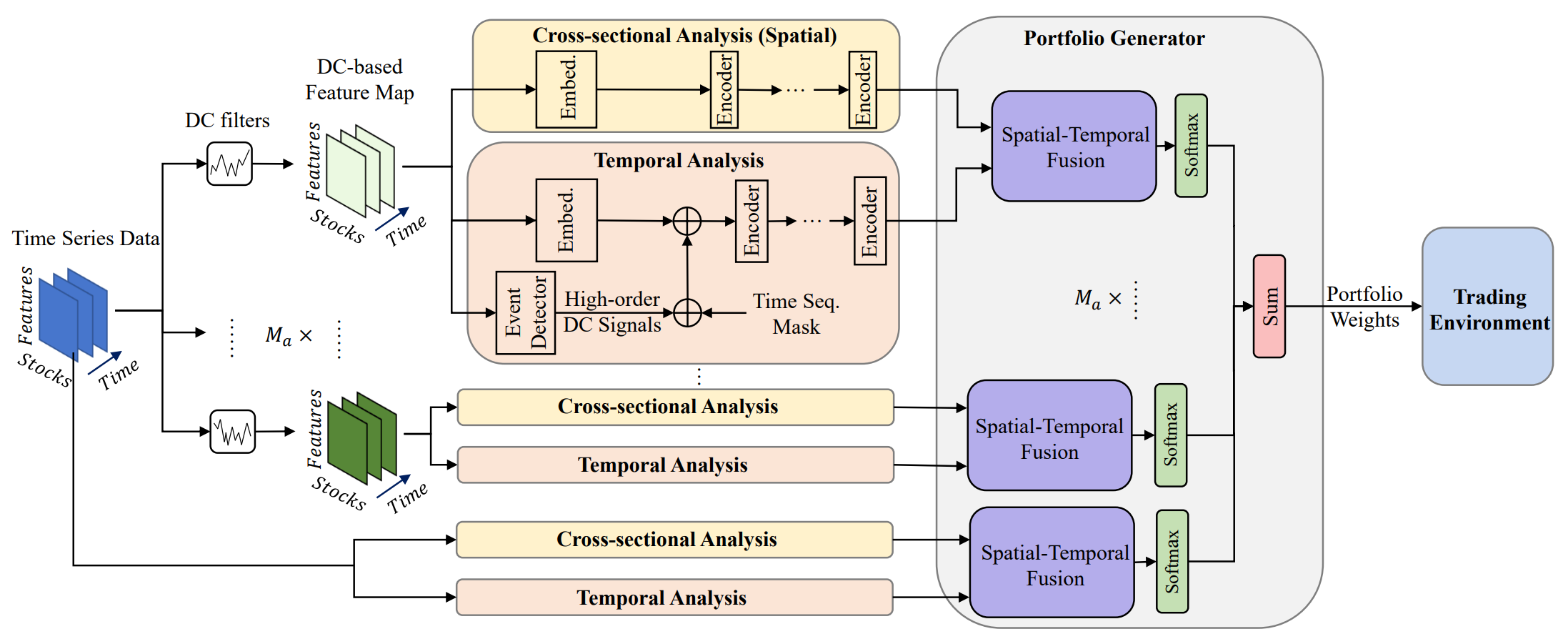
The MASAAT framework exhibits a clearly defined modular architecture. This makes it possible to implement each module as an independent class and then integrate the resulting objects into a unified structure. In the previous article, we introduced the implementation algorithms for the multi-agent object CNeuronPLRMultiAgentsOCL, which transforms the analyzed multimodal time series into multi-scale piecewise-linear representations. We also reviewed the algorithm of the CSACNeuronCrossSectionalAnalysis module. In this article, we continue this line of work.

Time Analysis Module

We concluded the previous article with an examination of the CNeuronCrossSectionalAnalysis object, which implements the CSA module. Alongside it, the MASAAT framework includes the temporal analysis module (TA). It is designed to uncover dependencies between individual time points within the analyzed multimodal sequence. A closer look at the structures of these two modules reveals their near-complete similarity. However, they perform cross-analysis of the original data. In other words, they effectively analyze the sequence from different perspectives.

This naturally suggests a straightforward solution: transposing the original sequence before feeding it into the previously developed CNeuronCrossSectionalAnalysis object. At this point, however, we face the need to transpose two dimensions within a three-dimensional tensor. It is important to recall that we aim to perform parallel analysis of several multimodal time sequences. More precisely, each agent processes its own scale of the piecewise-linear representation of the source multimodal sequence. Consequently, the input to the object is expected to be a 3D tensor in the form [Agent, Asset, Time]. For the purposes of analyzing dependencies across time points, we must transpose the last two dimensions. Since our library does not yet support this functionality, it must be implemented.

There are multiple ways to approach the transposition of a three-dimensional tensor across the last two dimensions. The most direct solution would be to develop a new kernel within the OpenCL program, followed by creating a new class in the main program to manage this kernel. This approach is likely the most efficient in terms of computational performance. However, it is also the most labor-intensive for the developer. To reduce programming complexity at the expense of computational resources, we instead opted to implement the process using three sequentially applied transposition layers that were previously created. More specifically, first, we apply a 2D matrix transposition layer by merging the last two dimensions into one:

[Agent, [Asset, Time]] → [[Time, Asset], Agent]

Next, we use the CNeuronTransposeRCDOCL object to transpose the three-dimensional tensor across the first two dimensions:

[Time, Asset, Agent] → [Asset, Time, Agent]

Finally, we apply another 2D matrix transposition layer to restore the agent dimension to the first position by merging the other two dimensions into one:

[[Asset, Time], Agent] → [Agent, [Time, Asset]]

This process is implemented within the new class CNeuronTransposeVRCOCL, the structure of which is shown below.

class CNeuronTransposeVRCOCL  :  public CNeuronTransposeOCL
  {
protected:
   CNeuronTransposeOCL     cTranspose;
   CNeuronTransposeRCDOCL  cTransposeRCD;
   //---
   virtual bool      feedForward(CNeuronBaseOCL *NeuronOCL) override;
   virtual bool      calcInputGradients(CNeuronBaseOCL *prevLayer) override;

public:
                     CNeuronTransposeVRCOCL(void) {};
                    ~CNeuronTransposeVRCOCL(void) {};
   //---
   virtual bool      Init(uint numOutputs, uint myIndex, COpenCLMy *open_cl, 
                          uint variables, uint count, uint window, 
                          ENUM_OPTIMIZATION optimization_type, uint batch);
   //---
   virtual int       Type(void)  const override    {  return defNeuronTransposeVRCOCL; }
   //---
   virtual bool      Save(int const file_handle) override;
   virtual bool      Load(int const file_handle) override;
   virtual void      SetOpenCL(COpenCLMy *obj) override;
  };

As the parent object, we employ the two-dimensional matrix transposition layer, which simultaneously performs the final stage of data permutation. This design allows us to declare only two static objects within the body of the new class. Initialization of all objects is handled in the Init method, which receives all three dimensions of the tensor to be transposed as parameters.

bool CNeuronTransposeVRCOCL::Init(uint numOutputs, uint myIndex, COpenCLMy *open_cl,
                                  uint variables, uint count, uint window,
                                  ENUM_OPTIMIZATION optimization_type, uint batch)
  {
   if(!CNeuronTransposeOCL::Init(numOutputs, myIndex, open_cl, count * window, variables, optimization_type, batch))
      return false;

Within this method, we call the parent class method of the same name. However, it is important to note that the parent object is used exclusively for the final data rearrangement. Therefore, when invoking the parent method, we must supply the correct parameters. Specifically, the first dimension is defined as the product of the last two dimensions of the original tensor. The remaining dimension is straightforward.

After successfully executing the parent class method, we proceed to initialize the internal objects. First, we initialize the primary matrix transposition layer. Its parameters are the inverse of those provided earlier to the parent class.

   if(!cTranspose.Init(0, 0, OpenCL, variables, count * window, optimization, iBatch))
      return false;

Next, we initialize the object responsible for transposing the first two dimensions of the three-dimensional tensor. This step effectively swaps the asset and time dimensions.

   if(!cTransposeRCD.Init(0, 1, OpenCL, count, window, variables, optimization, iBatch))
      return false;
//---
   return true;
  }

Finally, we return the logical result of these operations to the calling program, concluding the method execution.

The initialization method presented here is straightforward and easy to follow. The same can be said about the other methods of this three-dimensional tensor transposition class. For example, in the feedForward method, we sequentially invoke the corresponding methods of the internal objects, with the process finalized by the parent class method of the same name.

bool CNeuronTransposeVRCOCL::feedForward(CNeuronBaseOCL *NeuronOCL)
  {
   if(!cTranspose.FeedForward(NeuronOCL))
      return false;
   if(!cTransposeRCD.FeedForward(cTranspose.AsObject()))
      return false;
//---
   return CNeuronTransposeOCL::feedForward(cTransposeRCD.AsObject());
  }

The algorithms for the backward-pass methods are provided separately in the attachment. Since this object does not contain trainable parameters, we will not examine them in detail here.

Now that we have the necessary data transposition object, we can proceed to the implementation of the temporal analysis module (TA), whose algorithms are implemented in the CNeuronTemporalAnalysis class. The functionality of this new class is deliberately simple. We transpose the input data and then apply the mechanisms of the cross-sectional attention (CSA) module. The structure of the new object is presented below.

class CNeuronTemporalAnalysis :  public CNeuronCrossSectionalAnalysis
  {
protected:
   CNeuronTransposeVRCOCL  cTranspose;
   //---
   virtual bool      feedForward(CNeuronBaseOCL *NeuronOCL) override;
   virtual bool      calcInputGradients(CNeuronBaseOCL *prevLayer) override;
   virtual bool      updateInputWeights(CNeuronBaseOCL *NeuronOCL) override;

public:
                     CNeuronTemporalAnalysis(void) {};
                    ~CNeuronTemporalAnalysis(void) {};
   //---
   virtual bool      Init(uint numOutputs, uint myIndex, COpenCLMy *open_cl,
                          uint window, uint window_key, uint heads, uint heads_kv,
                          uint units_count, uint layers, uint layers_to_one_kv,
                          uint variables, ENUM_OPTIMIZATION optimization_type, uint batch) override;
   //---
   virtual int       Type(void)   const override   {  return defNeuronTemporalAnalysis;   }
   //---
   virtual bool      Save(int const file_handle) override;
   virtual bool      Load(int const file_handle) override;
   virtual bool      WeightsUpdate(CNeuronBaseOCL *source, float tau) override;
   virtual void      SetOpenCL(COpenCLMy *obj) override;
  };

As the parent class, we use the cross-sectional attention module. As noted earlier, the functionality of this module forms the foundation of our algorithm. We only add an internal object for transposing the three-dimensional tensor across its last two dimensions. Initialization of the new and inherited objects is performed in the Init method, which mirrors the parameter structure of its parent class counterpart.

bool CNeuronTemporalAnalysis::Init(uint numOutputs, uint myIndex, COpenCLMy *open_cl,
                                   uint window, uint window_key, uint heads, uint heads_kv,
                                   uint units_count, uint layers, uint layers_to_one_kv, uint variables,
                                   ENUM_OPTIMIZATION optimization_type, uint batch)
  {
   if(!CNeuronCrossSectionalAnalysis::Init(numOutputs, myIndex, open_cl, 3 * units_count, window_key, heads, heads_kv,
                                           window / 3, layers, layers_to_one_kv, variables, optimization_type, batch))
      return false;

Inside this method, we immediately call the parent's initialization method, passing along all received parameters.

At this point, several nuances of our implementation should be noted. First, the external parameters specify the dimensions of the original data. Recall that we plan to transpose the three-dimensional tensor across its last two dimensions. Therefore, when passing parameters to the parent class initialization method, we swap the corresponding dimensions.

Second, we must consider the structure of the input data. This object receives the output of the multi-agent trend detection block. Accordingly, the model input consists of a tensor representing the piecewise-linear approximation of the multimodal time series. In our implementation, each directed segment of a univariate time series is represented by three elements. Logically, these should be treated as a single unit during analysis. Thus, we triple the analysis window size and, correspondingly, reduce the sequence length by a factor of three.

After the parent class initialization is successfully completed, we invoke the initialization method of the internal three-dimensional tensor transposition object.

   if(!cTranspose.Init(0, 0, OpenCL,variables, units_count, window, optimization_type, batch))
      return false;
//---
   return true;
  }

We then finalize the method by returning the logical result of the operations to the calling program.

The feed-forward and backpropagation algorithms of the CNeuronTemporalAnalysis object are quite simple. Therefore, we will not dwell on it in this article. The full source code for this class and all of its methods can be found in the attachment to this article.

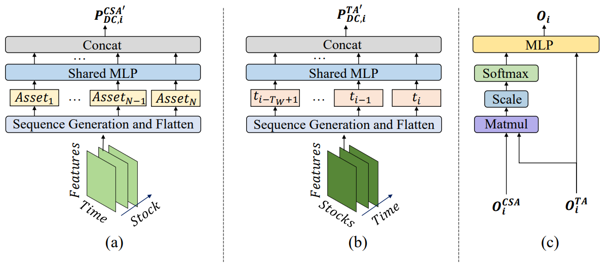
Portfolio Generation Module

At the output of the CSA and TA blocks, we obtain data enriched with information on asset-to-asset and time-to-time dependencies, respectively. This information is combined via an attention mechanism, enabling each agent to construct its own version of an investment portfolio. More precisely, each agent first forms asset embeddings that account for temporal dependencies. These embeddings are then passed through a fully connected layer to generate a weight vector representing the portfolio allocation, where the sum of all vector elements equals 1.

The mathematical representation of the portfolio generation function is as follows:

Based on the portfolio proposals, a final portfolio representation is constructed.

Here we diverge slightly from the authors’ original presentation of the MASAAT framework. However, this deviation is more logical than mathematical in nature. In practice, while closely following the original function, we reinterpret the resulting outputs.

Our task differs somewhat from that of the MASAAT authors. At the model's output, we aim to obtain an agent's action vector that specifies trade direction, position size, and stop-loss and take-profit levels. To determine position size, we require account state information in addition to the financial instrument dynamics, but this information is absent from the input data. Therefore, in our implementation of MASAAT, we expect the output to be a hidden state embedding that encapsulates a comprehensive analysis of the current market situation.

The final functionality of MASAAT is realized within the CNeuronPortfolioGenerator object, whose structure is shown below.

class CNeuronPortfolioGenerator  :  public CNeuronBaseOCL
  {
protected:
   uint              iAssets;
   uint              iTimePoints;
   uint              iAgents;
   uint              iDimension;
   //---
   CNeuronBaseOCL          cAssetTime[2];
   CNeuronTransposeVRCOCL  cTransposeVRC;
   CNeuronSoftMaxOCL       cSoftMax;
   //---
   virtual bool      feedForward(CNeuronBaseOCL *NeuronOCL) override { return false; }
   virtual bool      feedForward(CNeuronBaseOCL *NeuronOCL, CBufferFloat *SecondInput)  override;
   virtual bool      calcInputGradients(CNeuronBaseOCL *prevLayer) override { return false; }
   virtual bool      calcInputGradients(CNeuronBaseOCL *NeuronOCL, CBufferFloat *SecondInput, 
                                                                   CBufferFloat *SecondGradient, 
                                                ENUM_ACTIVATION SecondActivation = None) override;
   virtual bool      updateInputWeights(CNeuronBaseOCL *NeuronOCL) override;

public:
                     CNeuronPortfolioGenerator(void) {};
                    ~CNeuronPortfolioGenerator(void) {};
   //---
   virtual bool      Init(uint numOutputs, uint myIndex, COpenCLMy *open_cl,
                          uint assets, uint time_points, uint dimension,
                          uint agents,  uint projection,
                          ENUM_OPTIMIZATION optimization_type, uint batch);
   //---
   virtual int       Type(void)   const override   {  return defNeuronPortfolioGenerator;   }
   //---
   virtual bool      Save(int const file_handle) override;
   virtual bool      Load(int const file_handle) override;
   virtual bool      WeightsUpdate(CNeuronBaseOCL *source, float tau) override;
   virtual void      SetOpenCL(COpenCLMy *obj) override;
  };

Within the structure of this new class, we declare several internal objects, whose functions will be described during the method implementations. All internal objects are declared statically, allowing us to leave the class constructor and destructor empty. The initialization of these declared and inherited internal objects is performed in the Init method. Please note some nuances here.

bool CNeuronPortfolioGenerator::Init(uint numOutputs, uint myIndex, COpenCLMy *open_cl,
                                     uint assets, uint time_points, uint dimension,
                                     uint agents, uint projection,
                                     ENUM_OPTIMIZATION optimization_type, uint batch)
  {
   if(assets <= 0 || time_points <= 0 || dimension <= 0 || agents <= 0)
      return false;

The method receives several parameters, which require clarification:

• assets — the number of assets analyzed in the CSA module;
• time_points — the number of time points analyzed in the TA module;
• dimension — the embedding vector size for each element of the analyzed sequence (common to both CSA and TA modules);
• agents — the number of agents;
• projection — the projection size of the analyzed state at the module output.

Inside the method, we first validate the parameter values. All of them must be greater than zero. We then call the parent class initialization method, passing the projection size of the analyzed state. It corresponds to the tensor expected at the module's output.

   if(!CNeuronBaseOCL::Init(numOutputs, myIndex, open_cl, projection, optimization_type, batch))
      return false;

After successfully executing the parent class’s initialization, we store the external parameter values in internal variables.

   iAssets = assets;
   iTimePoints = time_points;
   iDimension = dimension;
   iAgents = agents;

We then proceed to initialize the internal objects. Referring back to the formula presented earlier, we note that the TA module output is used twice: once in its transposed form, and once in its original form.

Recall that the TA module outputs a three-dimensional tensor with dimensions [Agent, Time, Embedding]. Consequently, in this case, we must employ a three-dimensional tensor transposition object for the last two dimensions.

   if(!cTransposeVRC.Init(0, 0, OpenCL, iAgents, iTimePoints, iDimension, optimization, iBatch))
      return false;

Next, we multiply the CSA module results by the transposed TA outputs. The matrix multiplication method is inherited from the parent class. To store the results, we initialize an internal fully connected layer.

   if(!cAssetTime[0].Init(0, 1, OpenCL, iAssets * iTimePoints * iAgents, optimization, iBatch))
      return false;
   cAssetTime[0].SetActivationFunction(None);

The resulting values are normalized using the Softmax function.

   if(!cSoftMax.Init(0, 2, OpenCL, cAssetTime[0].Neurons(), optimization, iBatch))
      return false;
   cSoftMax.SetHeads(iAssets * iAgents);

It should be emphasized that normalization is performed per asset, per agent. Therefore, the number of normalization heads equals the product of the number of assets and the number of agents.

The normalized coefficients serve as attention weights for each time point at the level of individual assets across agents. By multiplying this matrix of coefficients by the TA outputs, we obtain the embeddings of the analyzed assets. To store these embeddings, we initialize another fully connected layer.

   if(!cAssetTime[1].Init(Neurons(), 3, OpenCL, iAssets * iDimension * iAgents, optimization, iBatch))
      return false;
   cAssetTime[1].SetActivationFunction(None);
//---
   return true;
  }

To project the embeddings generated by all agents into a unified representation of the analyzed environment, we employ a fully connected layer. Here it is important to note that this fully connected layer is the parent object of our class. Based on this fact, we avoid creating an additional internal layer, instead using the parent class functionality. In the final internal layer, we only specify the number of output connections corresponding to the projection size provided by the external program.

After successfully initializing all internal objects, we return the logical result of these operations to the calling program and conclude the method.

The next stage of our work involves developing the feed-forward algorithms in the feedForward method. It is important to note that in this case, we are dealing with two sources of input data. At the same time, we must remember that the results of the temporal analysis module are used twice. This circumstance compels us to designate this stream of information as the primary one.

bool CNeuronPortfolioGenerator::feedForward(CNeuronBaseOCL *NeuronOCL, CBufferFloat *SecondInput)
  {
   if(!SecondInput)
      return false;
//---
   if(!cTransposeVRC.FeedForward(NeuronOCL))
      return false;

Within the method, we first validate the pointer to the second data source and perform transposition on the first. After these preparatory steps, we proceed to the actual computations. First, we multiply the tensor from the second data source by the transposed tensor of the first.

   if(!MatMul(SecondInput, cTransposeVRC.getOutput(), cAssetTime[0].getOutput(), iAssets, iDimension, 
                                                                                 iTimePoints, iAgents))
      return false;

The results are normalized using the SoftMax function.

   if(!cSoftMax.FeedForward(cAssetTime[0].AsObject()))
      return false;

And then they are multiplied by the original data of the primary information stream.

   if(!MatMul(cSoftMax.getOutput(), NeuronOCL.getOutput(), cAssetTime[1].getOutput(), iAssets, iTimePoints,
                                                                                      iDimension, iAgents))
      return false;

Finally, using the parent class functionality, we project the obtained data into the specified subspace.

   return CNeuronBaseOCL::feedForward(cAssetTime[1].AsObject());
  }

The logical result of these operations is returned to the calling program, and the method concludes.

After completing the implementation of the feed-forward processes, we move on to the backpropagation algorithms. Here, we first examine the error gradient distribution method calcInputGradients.

bool CNeuronPortfolioGenerator::calcInputGradients(CNeuronBaseOCL *NeuronOCL, CBufferFloat *SecondInput, 
                                     CBufferFloat *SecondGradient, ENUM_ACTIVATION SecondActivation = -1)
  {
   if(!NeuronOCL || !SecondGradient || !SecondInput)
      return false;

The method parameters include pointers to the input data objects and the corresponding error gradients for both information streams. In the method body, we immediately verify the validity of the pointers. If the pointers are invalid, any further operations would be meaningless.

As you know, the propagation of error gradients follows the exact structure of the feed-forward information flow, only in reverse. The operations in this method begin with a call to the parent class’s method of the same name, propagating the gradient to the internal object.

   if(!CNeuronBaseOCL::calcInputGradients(cAssetTime[1].AsObject()))
      return false;

Next, we call the error gradient distribution method for the matrix multiplication operation, passing the data down to the input level and the internal Softmax layer.

   if(!MatMulGrad(cSoftMax.getOutput(), cSoftMax.getGradient(),
                  NeuronOCL.getOutput(), cTransposeVRC.getPrevOutput(),
                  cAssetTime[1].getGradient(),
                  iAssets, iTimePoints, iDimension, iAgents))
      return false;

However, it is important to remember that the error gradient for the input level of the primary information stream must arrive from two distinct flows. Therefore, the values obtained at this stage are stored in an auxiliary buffer of the data transposition object.

We then propagate the error gradient through the Softmax layer back to the level of the unnormalized coefficients.

   if(!cAssetTime[0].calcHiddenGradients(cSoftMax.AsObject()))
      return false;

Afterward, we distribute the resulting gradient to the second data source and to our transposition layer.

   if(!MatMulGrad(SecondInput, SecondGradient,
                  cTransposeVRC.getOutput(), cTransposeVRC.getGradient(),
                  cAssetTime[0].getGradient(),
                  iAssets, iDimension, iTimePoints, iAgents))
      return false;

At this point, we immediately check the activation function of the second data source and, if necessary, adjust the error gradient using the corresponding derivative.

   if(SecondActivation != None)
      if(!DeActivation(SecondInput, SecondGradient, SecondGradient, SecondActivation))
         return false;

At this stage, the gradient has been passed to the CSA module (which in this case serves as the second data source). What remains is to complete the transfer of the gradient to the temporal attention module (the primary information stream). This module receives gradients via two information flows: from the attention coefficients and directly from the results. The data from these two streams are currently stored in different buffers of the data transposition object. In the primary gradient buffer, we find the transposed values from the attention coefficient stream. Using the core functionality of the three-dimensional tensor transposition object, we propagate these values back to the input level.

   if(!NeuronOCL.calcHiddenGradients(cTransposeVRC.AsObject()) ||
      !SumAndNormilize(NeuronOCL.getGradient(), cTransposeVRC.getPrevOutput(), NeuronOCL.getGradient(),
                                                                        iDimension, false, 0, 0, 0, 1))
      return false;

Next, we sum the data from both information streams. Finally, we adjust the resulting gradient according to the derivative of the activation function of the primary stream.

   if(NeuronOCL.Activation() != None)
      if(!DeActivation(NeuronOCL.getOutput(), cTransposeVRC.getPrevOutput(), cTransposeVRC.getPrevOutput(), 
                                                                                   NeuronOCL.Activation()))
         return false;
//---
   return true;
  }

The method concludes by returning the logical result of the operations to the calling program.

As for the method responsible for updating the model's parameters, I suggest reviewing it independently. The full source code of the CNeuronPortfolioGenerator class and all of its methods is provided in the attachment.

Assembling the MASAAT Framework

We have already implemented the functionality of the individual MASAAT framework blocks and now it is time to assemble them into a unified structure. This integration is implemented in the CNeuronMASAAT class. For its parent object, we selected the CNeuronPortfolioGenerator created earlier, which represents the final block of our MASAAT implementation. This choice eliminates the need to declare this module as an internal object of the new class since all necessary functionality will be inherited. The structure of the new class is shown below.

class CNeuronMASAAT  :  public CNeuronPortfolioGenerator
  {
protected:
   CNeuronTransposeOCL              cTranspose;
   CNeuronPLRMultiAgentsOCL         cPLR;
   CNeuronBaseOCL                   cConcat;
   CNeuronCrossSectionalAnalysis    cCrossSectionalAnalysis;
   CNeuronTemporalAnalysis          cTemporalAnalysis;
   //---
   virtual bool      feedForward(CNeuronBaseOCL *NeuronOCL) override;
   virtual bool      feedForward(CNeuronBaseOCL *NeuronOCL, CBufferFloat *SecondInput)  override
     { return        feedForward(NeuronOCL); }
   virtual bool      calcInputGradients(CNeuronBaseOCL *prevLayer) override;
   virtual bool      calcInputGradients(CNeuronBaseOCL *NeuronOCL, CBufferFloat *SecondInput, 
                       CBufferFloat *SecondGradient, ENUM_ACTIVATION SecondActivation = None) override
     { return        calcInputGradients(NeuronOCL); }
   virtual bool      updateInputWeights(CNeuronBaseOCL *NeuronOCL) override;

public:
                     CNeuronMASAAT(void)  {};
                    ~CNeuronMASAAT(void)  {};
   //---
   //---
   virtual bool      Init(uint numOutputs, uint myIndex, COpenCLMy *open_cl,
                          uint window, uint window_key, uint heads, uint units_cout,
                          uint layers, vector<float> &min_distance, uint projection,
                          ENUM_OPTIMIZATION optimization_type, uint batch);
   //---
   virtual int       Type(void)   const override   {  return defNeuronMASAAT;   }
   //---
   virtual bool      Save(int const file_handle) override;
   virtual bool      Load(int const file_handle) override;
   virtual bool      WeightsUpdate(CNeuronBaseOCL *source, float tau) override;
   virtual void      SetOpenCL(COpenCLMy *obj) override;
  };

In this class structure, we see the declaration of all previously created objects. As you can see, the algorithms for all methods will be built upon sequentially calling the corresponding methods of the internal objects. The execution order will become clearer as we proceed with the method implementations.

All internal objects are declared statically, which allows us to leave the constructor and destructor of the class empty. The initialization of all declared and inherited objects is carried out in the Init method.

bool CNeuronMASAAT::Init(uint numOutputs, uint myIndex, COpenCLMy *open_cl,
                         uint window, uint window_key, uint heads, uint units_cout,
                         uint layers, vector<float> &min_distance, uint projection,
                         ENUM_OPTIMIZATION optimization_type, uint batch)
  {
   if(!CNeuronPortfolioGenerator::Init(numOutputs, myIndex, open_cl, window, units_cout / 3,
                                       window_key, (uint)min_distance.Size() + 1, projection, optimization_type, batch))
      return false;

The parameters of this method include the key constants that describe the structure of the input data and define the architecture of the object being initialized.

In the method body, and following established practice, we immediately call the parent class initialization method, which already contains the logic for initializing inherited objects and basic interfaces. However, it is worth noting that in this case, we employ the parent class as a fully functional block within the broader algorithm. This module is used as the final output of our MASAAT implementation. Therefore, we must look slightly ahead to determine the correct initialization parameters for the parent object.

At the input of the parent object, we plan to supply the results of the CSA and TA modules. For these modules, the number of analyzed assets equals the input window size, while the number of time points corresponds to the length of the input sequence. But wait — we are applying a transformation of the original multimodal time series into its piecewise-linear representation. This means the number of time points will be reduced by a factor of three. Consequently, when passing parameters to the parent class initialization method, we divide the length of the original sequence by three.

Examining the parameters further, we arrive at the number of agents. As discussed earlier, in building the multi-agent transformation object, the number of agents is determined by the length of the vector of threshold deviations. However, if we consider the MASAAT authors' analysis of individual framework components, we find that combining the piecewise-linear representation of a time series with the original series improves model efficiency. Therefore, we increase the number of agents by one, assigning the additional agent to work with the unmodified original time series.

All other parameters are passed unchanged.

Once the parent class initialization has been successfully executed, we proceed to initialize the newly declared objects. First, we initialize the data transposition object.

   if(!cTranspose.Init(0, 0, OpenCL, units_cout, window, optimization, iBatch))
      return false;

Next, we initialize the multi-agent transformation object that generates the piecewise-linear representations of the analyzed sequence.

   if(!cPLR.Init(0, 1, OpenCL, window, units_cout, false, min_distance, optimization, iBatch))
      return false;

The transformation results are concatenated with the original data. For this, we initialize a fully connected layer of the corresponding size.

   if(!cConcat.Init(0, 2, OpenCL, cTranspose.Neurons() + cPLR.Neurons(), optimization, iBatch))
      return false;

Finally, we initialize the CSA and TA modules. Both operate on the same source data and therefore receive identical parameters.

   if(!cCrossSectionalAnalysis.Init(0, 3, OpenCL, units_cout, window_key, heads, heads / 2, window, layers, 1, 
                                                                                 iAgents, optimization, iBatch))
      return false;
   if(!cTemporalAnalysis.Init(0, 4, OpenCL, units_cout, window_key, heads, heads / 2, window, layers, 1, 
                                                                                  iAgents, optimization, iBatch))
      return false;
//---
   return true;
  }

After successfully initializing all internal objects, we return the logical result of the operations to the calling program and conclude the method.

We now proceed to the forward-pass algorithm within the feedForward method. Everything is quite simple here. The method parameters provide a pointer to the input data object, which we immediately pass to the transposition object's method of the same name.

bool CNeuronMASAAT::feedForward(CNeuronBaseOCL *NeuronOCL)
  {
   if(!cTranspose.FeedForward(NeuronOCL))
      return false;

The resulting data are then transformed into several versions of the piecewise-linear time series representation, and the outputs are concatenated with the original data, albeit in transposed form.

   if(!cPLR.FeedForward(cTranspose.AsObject()))
      return false;
   if(!Concat(cTranspose.getOutput(), cPLR.getOutput(), cConcat.getOutput(), cTranspose.Neurons(), cPLR.Neurons(), 1))
      return false;

The prepared data are subsequently passed to the CSA and TA modules, with their outputs then supplied to the parent class corresponding method.

   if(!cCrossSectionalAnalysis.FeedForward(cConcat.AsObject()))
      return false;
   if(!cTemporalAnalysis.FeedForward(cConcat.AsObject()))
      return false;
//---
   return CNeuronPortfolioGenerator::feedForward(cTemporalAnalysis.AsObject(), cCrossSectionalAnalysis.getOutput());
  }

The method then concludes by returning the logical result of the operation to the caller.

Behind the apparent simplicity of the forward-pass method lies a complex branching of information flows. Notice that the transposed original data and the concatenated tensor are both used twice. This leads to complications in the organization of error gradient distribution within the calcInputGradients method.

In the parameters of this method, we receive a pointer to the input data object, which must receive the error gradient. And in the method body, we immediately check the relevance of the received pointer.

bool CNeuronMASAAT::calcInputGradients(CNeuronBaseOCL *prevLayer)
  {
   if(!prevLayer)
      return false;

Afterward, we invoke the parent class method of the same name to distribute the error gradient between the CSA and TA modules according to their influence on the model output.

   if(!CNeuronPortfolioGenerator::calcInputGradients(cTemporalAnalysis.AsObject(),
         cCrossSectionalAnalysis.getOutput(),
         cCrossSectionalAnalysis.getGradient(),
         (ENUM_ACTIVATION)cCrossSectionalAnalysis.Activation()))
      return false;

Both modules operate on the concatenated tensor. Therefore, the gradient must be propagated to this tensor from two different streams. First, we pass the gradient from one module.

   if(!cConcat.calcHiddenGradients(cCrossSectionalAnalysis.AsObject()))
      return false;

Then, by applying a buffer substitution technique, we retrieve the gradient values from the second stream, subsequently summing the information from both sources.

   CBufferFloat *grad = cConcat.getGradient();
   if(!cConcat.SetGradient(cConcat.getPrevOutput(), false) ||
      !cConcat.calcHiddenGradients(cTemporalAnalysis.AsObject()) ||
      !SumAndNormilize(grad, cConcat.getGradient(), grad, 1, 0, 0, 0, 0, 1) ||
      !cConcat.SetGradient(grad, false))
      return false;

The gradient of the concatenated tensor is then distributed among the concatenated objects. At this point, we must remember that the data transposition object is expected to receive its gradient via a different stream. Thus, we employ an auxiliary data buffer at this stage.

   if(!DeConcat(cTranspose.getPrevOutput(), cPLR.getGradient(), cConcat.getGradient(), cTranspose.Neurons(), 
                                                                                         cPLR.Neurons(), 1))
      return false;

Before continuing with the gradient distribution among objects, we verify whether the correction by the activation function derivative is necessary.

   if(cPLR.Activation() != None)
      if(!DeActivation(cPLR.getOutput(), cPLR.getGradient(), cPLR.getGradient(), cPLR.Activation()))
         return false;

Next, we propagate the gradient through the multi-agent piecewise-linear transformation object and sum the values from both streams.

   if(!cTranspose.calcHiddenGradients(cPLR.AsObject()) ||
      !SumAndNormilize(cTranspose.getGradient(), cTranspose.getPrevOutput(), cTranspose.getGradient(), iDimension, 
                                                                                               false, 0, 0, 0, 1))
      return false;

If required, we adjust the gradient according to the activation function derivative and then pass it back to the input level.

   if(cTranspose.Activation() != None)
      if(!DeActivation(cTranspose.getOutput(), cTranspose.getGradient(), cTranspose.getGradient(), 
                                                                         cTranspose.Activation()))
         return false;
   if(!prevLayer.calcHiddenGradients(cTranspose.AsObject()))
      return false;
//---
   return true;
  }

Finally, the method concludes by returning the logical result of the operations to the calling program.

At this point, we conclude our examination of the algorithmic implementation of MASAAT approaches. The full source code for all presented classes and methods can be found in the attachment. There, you will also find all the programs used in preparing this article, as well as the model architectures. We will briefly touch upon the model architectures. Our MASAAT framework implementation was integrated into the Actor model. We will not examine the full architecture here. It is almost entirely inherited from our previous works. Instead, let us look at the declaration of the new layer.

In the dynamic array of window sizes, we specify the size of the analyzed data window and the length of the hidden state tensor produced by the output layer. 

//--- layer 2
   if(!(descr = new CLayerDescription()))
      return false;
   descr.type = defNeuronMASAAT;
//--- Windows
     {
      int temp[] = {BarDescr, LatentCount};
      if(ArrayCopy(descr.windows, temp) < (int)temp.Size())
         return false;
     }

The threshold values for our three agents were generated as a geometric progression.

//--- Min Distance
     {
      vector<float> ones = vector<float>::Ones(3);
      vector<float> cs = ones.CumSum() - 1;
      descr.radius = pow(ones * 2, cs) * 0.01f;
     }

All other parameters retain their standard values.

   descr.window_out = 32;
   descr.count = HistoryBars;
   descr.step = 4;               //Heads
   descr.layers = 3;             //Layers
   descr.batch = 1e4;
   descr.activation = None;
   descr.optimization = ADAM;
   if(!actor.Add(descr))
     {
      delete descr;
      return false;
     }

The full architecture of the models, as mentioned earlier, is available in the attachment.

Test

Our work on implementing the MASAAT framework approaches in MQL5 has reached its logical conclusion. We now proceed to the most important stage - evaluating the effectiveness of the implemented methods on real historical data.

It is important to emphasize that we are assessing the *implemented* approaches, not the MASAAT framework in its original form. This is because modifications were introduced during implementation.

The models were trained on historical data from 2023 for EURUSD, with an H1 timeframe. All analyzed indicators were used with their default parameter settings.

For the initial training stage, we used a dataset collected in the course of earlier studies, which was periodically updated during training to adapt to the Actor's current strategy.

After several cycles of training and dataset updates, we obtained a policy that demonstrated profitability on both the training and testing datasets.

Final testing of the trained policy was conducted on historical data from January 2024, with all other parameters held constant. The test results are presented below.

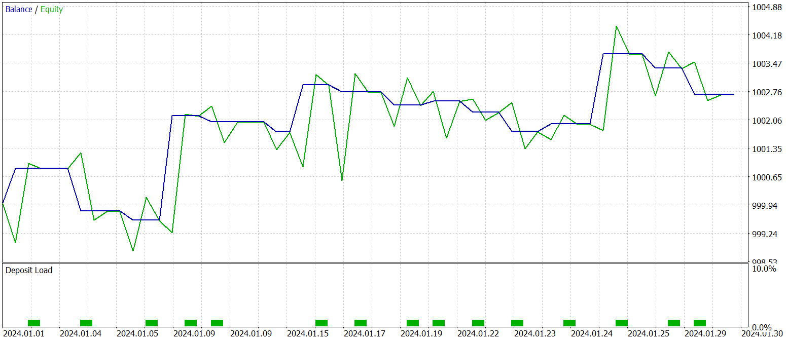
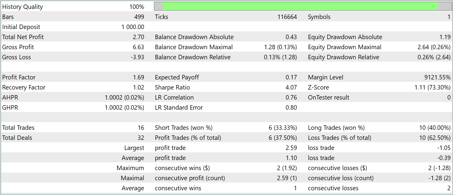
As the data show, the model executed 16 trades during the test period. Slightly more than one-third of them closed in profit. However, the maximum profitable trade exceeded the largest loss by a factor of 2.5. Moreover, the average profit per trade was three times higher than the average loss. As a result, we observe a clear upward trend in account balance.

Conclusion

In this work, we examined the multi-agent adaptive MASAAT framework, designed for investment portfolio optimization. MASAAT combines attention mechanisms with time-series analysis. The framework employs an ensemble of trading agents to perform multifaceted analysis of price data, thereby reducing bias in trading decisions. Each agent applies an attention-based cross-sectional analysis mechanism to identify correlations between assets and time points within the observation period. This information is then merged using a spatiotemporal fusion module, enabling effective data integration and enhancing trading strategies.

In the practical part, we implemented our own interpretation of the proposed methods using MQL5. We integrated these approaches into a model and trained it on real historical data. The testing results of the trained model demonstrate the potential of the proposed methods.

References

• Developing An Attention-Based Ensemble Learning Framework for Financial Portfolio Optimisation
• Other articles from this series

Programs used in the article

#	Name	Type	Description
1	Research.mq5	Expert Advisor	Expert Advisor for collecting samples
2	ResearchRealORL.mq5	Expert Advisor	Expert Advisor for collecting samples using the Real-ORL method
3	Study.mq5	Expert Advisor	Model training Expert Advisor
4	Test.mq5	Expert Advisor	Model testing Expert Advisor
5	Trajectory.mqh	Class library	System state description structure
6	NeuroNet.mqh	Class library	A library of classes for creating a neural network
7	NeuroNet.cl	Code Base	OpenCL program code library