
Neural networks made easy (Part 62): Using Decision Transformer in hierarchical models

Introduction
While solving real problems, we often encounter the problem of stochastic and dynamically changing environments, which forces us to look for new adaptive algorithms. In recent decades, significant efforts have been devoted to developing reinforcement learning (RL) techniques that can train agents to adapt to a variety of environments and tasks. However, the application of RL in real world faces a number of challenges, including offline learning in variable and stochastic environments, as well as the difficulties of planning and control in high-dimensional spaces of states and actions.
Very often, when solving complex problems, the most efficient way is to divide one problem into its constituent subtasks. We talked about the advantages of this approach when considering hierarchical methods. Such integrated approaches allow the creation of more adaptive models.
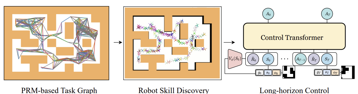
Previously, we considered hierarchical models for solving problems with, so to speak, the classical approach of the Markov process. However, the advantages of using hierarchical approaches also apply to sequence analysis problems. One such algorithm is the Control Transformer presented in the article "Control Transformer: Robot Navigation in Unknown Environments through PRM-Guided Return-Conditioned Sequence Modeling". The method authors position it as a new architecture designed to solve complex control and navigation problems based on reinforcement learning. This method combines modern methods of reinforcement learning, planning and machine learning, which allows us to create adaptive control strategies in a variety of environments.
Control Transformer opens new perspectives for solving complex control problems in robotics, autonomous driving and other fields. I propose to look at the prospects for using this method in solving our trading problems.
1. Control Transformer algorithm
The Control Transformer algorithm is a rather complex method and includes several separate blocks, which, in fact, is characteristic of hierarchical models. It should also be said that the algorithm was developed to navigate and control the behavior of robots. Therefore, the algorithm description is presented in this context.
To solve the problem of control over a long planning horizon, the authors of the method propose to decompose it into smaller subtasks in the form of certain segments of a limited distance. The method authors use Probabilistic Road Maps to build the G, in which the vertices are points and the edges indicate the ability to move between connected points using a local scheduler. The graph is constructed based on the sample of n random points in the environment, which are subsequently connected to neighboring points at a distance of no more than d (hyperparameter) forming an edge in the graph provided that there is a path between the points.
Thus, in the resulting G graph, we can reach any Xg target point from any X0 starting point. This is achieved by searching the graph for the nearest neighbors of the starting and target points. Then we obtain a sequence of waypoints (trajectory) using the shortest path search algorithm. After that, the robot can move from the initial state to the goal, executing the actions of the πc local controller policy. A sequence of waypoints or plan that guides the πc policy can be fixed or updated as the robot progresses.
In order to train the πc local policy, the method authors used reinforcement learning method aimed at achieving the goal (GCRL). In this case, the problem is modeled using a Markov decision-making process with a condition directed at the goal. It is suggested that sample-based planning can be used to set goals and train strategies.
To do this, we first use Probabilistic Road Maps to obtain the G graph as described above. Next, for each learning episode, an edge is selected from the graph. The edge serves as the beginning and goal for this episode. This process is compatible with any goal-based learning algorithm. The authors used Soft Actor-Critic in their experiments with dense rewards proportional to progress toward a goal. Low-level strategies can be trained efficiently because the state space of strategies only contains information about their own position and they do not need to learn to avoid the constraint.
After training the πc local policy, we need to arrange a process that will guide it to achieve the global goal. In other words, we have to train a model that generates planned trajectories. The goals and rewards of this model are set in relation to the end goal, not the waypoints followed by πc. Obviously, to achieve the global goals of the model, more initial data is required. High-dimensional observations and other available information are added to the low-dimensional local state data. For example, it may be a local map.
To train a model on data collected using sampling-based design, we consider a sequence modeling problem, including orientation towards achieving the goal. In their work, the method authors also consider a partially observable multi-task environment, in which the strategy can work in several environments with the same navigation task, but with a different structure for each environment. Although it is possible to learn autoregressive action prediction on this sequence, we encounter some problems. As in DT, the optimal RTG is assumed to be constant because we do not know the optimal initial predictive reward, which depends on the unknown structure of the environment. It may change in different episodes. It also depends on initial states and goal positions. Therefore, we need to explore changes that will allow DT to generalize to unknown environments, working from any starting position to any goal.
One approach is to train the full RTG distribution from offline data. Then we need to select conditions from this distribution during operation. However, it is difficult to train the complete distribution of RTGs in a goal-oriented task so that one can generalize and predict RTGs in unknown environments. Instead, the method authors propose to train the average value function for this distribution. The function estimates the expected reward at the S point for a given goal g within the T trajectory. This function is also not based on past history, since at the moment of start of operation we predict the initial expected reward R̃0. Next, we adjust the RTG to the actual reward from the environment. The value function is parameterized as a separate neural network and is trained using MSE.
To obtain more optimal behavior, we can adjust the trained value by a certain constant ratio. In addition, it is possible to train the value function only on the best trajectories or on those that satisfy some predefined condition.
The author's visualization of the Control Transformer method is presented below.
One of the common problems with offline learning is distribution shift when the trained strategy is put into practice and the actual distribution of trajectories does not match the distribution of the training set. This may cause errors to accumulate and lead to situations where the strategy becomes suboptimal. To solve this problem, the method authors propose to expand the training set after the offline training stage using the current model policy and fine-tune the models offline afterwards.
2. Implementation using MQL5
After considering the theoretical aspects of the Control Transformer method, we move on to its implementation using MQL5. As mentioned earlier, the algorithm is complex. Therefore, during the implementation process, we will use the developments from a number of previous articles. The first thing we started considering the method with was constructing a graph of possible movements.
2.1. Collection of training set
In our case of a stochastic environment and a continuous action space, constructing such a graph may be a non-trivial task. We decided to approach the problem from the other side and use experience gained while developing the Go-Explore method. We have made minor adjustments to the "...\CT\Faza1.mq5" EA and collected possible trajectories of trading operations within the training period. While doing this, we selected trajectories with maximum profitability.
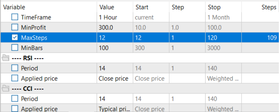
To do this, we added the maximum number of sampled actions and the minimum trajectory length in the EA external parameters. The appearance of these parameters is caused by a rather low probability (close to “0”) of sampling an acceptable trajectory over the entire training interval in one pass. It is much more likely to gradually sample small areas with profitable transactions, which are then collected into a common profitable sequence of actions.
input int                  MaxSteps    =  48;
input int                  MinBars     =  20;
Let me remind you right away that the EA does not use neural network models. All actions are sampled from a uniform distribution.
In the EA initialization method, we first initialize the indicator and trading operation class objects.
//+------------------------------------------------------------------+
//| Expert initialization function                                   |
//+------------------------------------------------------------------+
int OnInit()
  {
//---
   if(!Symb.Name(_Symbol))
      return INIT_FAILED;
   Symb.Refresh();
//---
   if(!RSI.Create(Symb.Name(), TimeFrame, RSIPeriod, RSIPrice))
      return INIT_FAILED;
//---
   if(!CCI.Create(Symb.Name(), TimeFrame, CCIPeriod, CCIPrice))
      return INIT_FAILED;
//---
   if(!ATR.Create(Symb.Name(), TimeFrame, ATRPeriod))
      return INIT_FAILED;
//---
   if(!MACD.Create(Symb.Name(), TimeFrame, FastPeriod, SlowPeriod, SignalPeriod, MACDPrice))
      return INIT_FAILED;
   if(!RSI.BufferResize(NBarInPattern) || !CCI.BufferResize(NBarInPattern) ||
      !ATR.BufferResize(NBarInPattern) || !MACD.BufferResize(NBarInPattern))
     {
      PrintFormat("%s -> %d", __FUNCTION__, __LINE__);
      return INIT_FAILED;
     }
//---
   if(!Trade.SetTypeFillingBySymbol(Symb.Name()))
      return INIT_FAILED;
We initialize the necessary variables and sample the trajectory and initial state to continue the previously saved trajectory. Of course, such sampling is only possible if there are previously saved trajectories.
   PrevBalance = AccountInfoDouble(ACCOUNT_BALANCE);
   PrevEquity = AccountInfoDouble(ACCOUNT_EQUITY);
   AgentResult = vector<float>::Zeros(NActions);
//---
   int error_code;
   if(Buffer.Size() > 0 || LoadTotalBase())
     {
      int tr = int(MathRand() / 32767.0 * Buffer.Size());
      Loaded = Buffer[tr];
      StartBar = MathMax(0,Loaded.Total - int(MathMax(Math::MathRandomNormal(0.5, 0.5, error_code), 0) * MaxSteps));
     }
//---
   return(INIT_SUCCEEDED);
  }
If there are no previously passed trajectories, the EA begins to sample actions from the first bar.
Direct data collection is carried out in the OnTick tick handling function. Here, as before, we check the occurrence of the opening event of a new bar and, if necessary, load historical data on the movement of the instrument and indicator parameters.
//+------------------------------------------------------------------+
//| Expert tick function                                             |
//+------------------------------------------------------------------+
void OnTick()
  {
//---
   if(!IsNewBar())
      return;
//---
   CurrentBar++;
   int bars = CopyRates(Symb.Name(), TimeFrame, iTime(Symb.Name(), TimeFrame, 1), NBarInPattern, Rates);
   if(!ArraySetAsSeries(Rates, true))
      return;
//---
   RSI.Refresh();
   CCI.Refresh();
   ATR.Refresh();
   MACD.Refresh();
   Symb.Refresh();
   Symb.RefreshRates();
We transfer the loaded data into the structure for setting into the experience playback buffer.
//--- History data
   float atr = 0;
   for(int b = 0; b < (int)NBarInPattern; b++)
     {
      float open = (float)Rates[b].open;
      float rsi = (float)RSI.Main(b);
      float cci = (float)CCI.Main(b);
      atr = (float)ATR.Main(b);
      float macd = (float)MACD.Main(b);
      float sign = (float)MACD.Signal(b);
      if(rsi == EMPTY_VALUE || cci == EMPTY_VALUE || atr == EMPTY_VALUE || macd == EMPTY_VALUE || sign == EMPTY_VALUE)
         continue;
      //---
      int shift = b * BarDescr;
      sState.state[shift] = (float)(Rates[b].close - open);
      sState.state[shift + 1] = (float)(Rates[b].high - open);
      sState.state[shift + 2] = (float)(Rates[b].low - open);
      sState.state[shift + 3] = (float)(Rates[b].tick_volume / 1000.0f);
      sState.state[shift + 4] = rsi;
      sState.state[shift + 5] = cci;
      sState.state[shift + 6] = atr;
      sState.state[shift + 7] = macd;
      sState.state[shift + 8] = sign;
     }
Add information about the account status and rewards from the environment.
//--- Account description
   sState.account[0] = (float)AccountInfoDouble(ACCOUNT_BALANCE);
   sState.account[1] = (float)AccountInfoDouble(ACCOUNT_EQUITY);
//---
   double buy_value = 0, sell_value = 0, buy_profit = 0, sell_profit = 0;
   double position_discount = 0;
   double multiplyer = 1.0 / (60.0 * 60.0 * 10.0);
   int total = PositionsTotal();
   datetime current = TimeCurrent();
   for(int i = 0; i < total; i++)
     {
      if(PositionGetSymbol(i) != Symb.Name())
         continue;
      double profit = PositionGetDouble(POSITION_PROFIT);
      switch((int)PositionGetInteger(POSITION_TYPE))
        {
         case POSITION_TYPE_BUY:
            buy_value += PositionGetDouble(POSITION_VOLUME);
            buy_profit += profit;
            break;
         case POSITION_TYPE_SELL:
            sell_value += PositionGetDouble(POSITION_VOLUME);
            sell_profit += profit;
            break;
        }
      position_discount += profit - (current - PositionGetInteger(POSITION_TIME)) * multiplyer * MathAbs(profit);
     }
   sState.account[2] = (float)buy_value;
   sState.account[3] = (float)sell_value;
   sState.account[4] = (float)buy_profit;
   sState.account[5] = (float)sell_profit;
   sState.account[6] = (float)position_discount;
   sState.account[7] = (float)Rates[0].time;
//---
   sState.rewards[0] = float((sState.account[0] - PrevBalance) / PrevBalance);
   sState.rewards[1] = float(sState.account[1] / PrevBalance - 1.0);
Redefine the internal variables.
   PrevBalance = sState.account[0];
   PrevEquity = sState.account[1];
Next we have to select the Agent's action. As mentioned above, we do not use models here. Instead, we check for the start of the sampling phase. When repeating a previously saved trajectory, we take the action from our trajectory. If the sampling period has arrived, then we generate an action vector from a uniform distribution.
   vector<float> temp = vector<float>::Zeros(NActions);
   if((CurrentBar - StartBar) < MaxSteps)
      if(CurrentBar < StartBar)
         temp.Assign(Loaded.States[CurrentBar].action);
      else
         temp = SampleAction(NActions);
The resulting action is performed in the environment.
//---
   double min_lot = Symb.LotsMin();
   double step_lot = Symb.LotsStep();
   double stops = MathMax(Symb.StopsLevel(), 1) * Symb.Point();
   if(temp[0] >= temp[3])
     {
      temp[0] -= temp[3];
      temp[3] = 0;
     }
   else
     {
      temp[3] -= temp[0];
      temp[0] = 0;
     }
   float delta = MathAbs(AgentResult - temp).Sum();
   AgentResult = temp;
//--- buy control
   if(temp[0] < min_lot || (temp[1] * MaxTP * Symb.Point()) <= stops || (temp[2] * MaxSL * Symb.Point()) <= stops)
     {
      if(buy_value > 0)
         CloseByDirection(POSITION_TYPE_BUY);
     }
   else
     {
      double buy_lot = min_lot + MathRound((double)(temp[0] - min_lot) / step_lot) * step_lot;
      double buy_tp = Symb.NormalizePrice(Symb.Ask() + temp[1] * MaxTP * Symb.Point());
      double buy_sl = Symb.NormalizePrice(Symb.Ask() - temp[2] * MaxSL * Symb.Point());
      if(buy_value > 0)
         TrailPosition(POSITION_TYPE_BUY, buy_sl, buy_tp);
      if(buy_value != buy_lot)
        {
         if(buy_value > buy_lot)
            ClosePartial(POSITION_TYPE_BUY, buy_value - buy_lot);
         else
            Trade.Buy(buy_lot - buy_value, Symb.Name(), Symb.Ask(), buy_sl, buy_tp);
        }
     }
//--- sell control
   if(temp[3] < min_lot || (temp[4] * MaxTP * Symb.Point()) <= stops || (temp[5] * MaxSL * Symb.Point()) <= stops)
     {
      if(sell_value > 0)
         CloseByDirection(POSITION_TYPE_SELL);
     }
   else
     {
      double sell_lot = min_lot + MathRound((double)(temp[3] - min_lot) / step_lot) * step_lot;;
      double sell_tp = Symb.NormalizePrice(Symb.Bid() - temp[4] * MaxTP * Symb.Point());
      double sell_sl = Symb.NormalizePrice(Symb.Bid() + temp[5] * MaxSL * Symb.Point());
      if(sell_value > 0)
         TrailPosition(POSITION_TYPE_SELL, sell_sl, sell_tp);
      if(sell_value != sell_lot)
        {
         if(sell_value > sell_lot)
            ClosePartial(POSITION_TYPE_SELL, sell_value - sell_lot);
         else
            Trade.Sell(sell_lot - sell_value, Symb.Name(), Symb.Bid(), sell_sl, sell_tp);
        }
     }
Interaction results are added to the experience playback buffer.
//---
   int shift = BarDescr * (NBarInPattern - 1);
   if((buy_value + sell_value) == 0)
      sState.rewards[2] -= (float)(atr / PrevBalance);
   else
      sState.rewards[2] = 0;
   for(ulong i = 0; i < NActions; i++)
      sState.action[i] = temp[i];
   if(!Base.Add(sState) || (CurrentBar - StartBar) >= MaxSteps)
      ExpertRemove();
//---
  }
Here we check that the maximum number of sampled steps has been reached and, if necessary, initiate the termination of the program.
A few words need to be said about changes in the method of adding trajectories to the experience playback buffer. While previously trajectories were added using the FIFO (first in, first out) method, now we save the most profitable passes. Therefore, after completing the next pass, we first check the size of our experience playback buffer.
//+------------------------------------------------------------------+
//| TesterPass function                                              |
//+------------------------------------------------------------------+
void OnTesterPass()
  {
//---
   ulong pass;
   string name;
   long id;
   double value;
   STrajectory array[];
   while(FrameNext(pass, name, id, value, array))
     {
      int total = ArraySize(Buffer);
      if(name != MQLInfoString(MQL_PROGRAM_NAME))
         continue;
      if(id <= 0)
         continue;
      if(total >= MaxReplayBuffer)
        {
When the buffer size limit is reached, we first search for the passage with the minimum profitability from the previously saved ones.
         for(int a = 0; a < id; a++)
           {
            float min = FLT_MAX;
            int min_tr = 0;
            for(int i = 0; i < total; i++)
              {
               float prof = Buffer[i].States[Buffer[i].Total - 1].account[1];
               if(prof < min)
                 {
                  min = MathMin(prof, min);
                  min_tr = i;
                 }
              }
We compare the profitability of the new pass with the minimum one in the experience playback buffer and, if necessary, set a new pass instead of the minimum one.
            float prof = array[a].States[array[a].Total - 1].account[1];
            if(min <= prof)
              {
               Buffer[min_tr] = array[a];
               PrintFormat("Replace %.2f to %.2f -> bars %d", min, prof, array[a].Total);
              }
           }
        }
This allows us to eliminate the costly sorting of data in the buffer. In one pass, we determine the minimum value and the feasibility of saving the new trajectory.
If the limit size of the experience playback buffer has not yet been reached, then we simply add a new pass and complete the method operation.
      else
        {
         if(ArrayResize(Buffer, total + (int)id, 10) < 0)
            return;
         ArrayCopy(Buffer, array, total, 0, (int)id);
        }
     }
  }
This concludes our introduction to the environmental interaction EA. You can find its full code in the attachment.
2.2. Skills training
The next step is to create a local policy training EA. The local policy plays the role of an executor, carrying out the instructions of a higher-level scheduler. In order to simplify the local policy model itself and in the spirit of hierarchical systems, we decided not to provide the current state of the environment as input to the model. In our vision, it will be a model that has a certain set of skills. The choice of skill to use is up to the scheduler. At the same time, the local policy model itself will not analyze the state of the environment.
To train skills, we will use the architecture of the auto encoder and the developments of the previously discussed hierarchical models. During training, we will randomly feed one skill into the input of our local policy model. The discriminator will try to identify the skill being used.
Here we have to determine the required number of skills to be trained. Here we also refer to our previous work. While considering clustering methods, we determined the optimal number of clusters in the range of 100-500. To avoid any skill shortage, we specify the size of the local policy input vector to be 512 elements.
#define WorkerInput 512
The architectures of the local policy and discriminator models are presented below. We did not overcomplicate these models. We expect to receive a one-hot vector or a vector of data normalized by the SoftMax function as input to the local policy model. Therefore, we did not add a batch normalization layer after the source data layer.
bool CreateWorkerDescriptions(CArrayObj *worker, CArrayObj *descriminator)
  {
//---
   CLayerDescription *descr;
//---
   if(!worker)
     {
      worker = new CArrayObj();
      if(!worker)
         return false;
     }
//--- Worker
   worker.Clear();
//--- Input layer
   if(!(descr = new CLayerDescription()))
      return false;
   descr.type = defNeuronBaseOCL;
   int prev_count = descr.count = WorkerInput;
   descr.activation = None;
   descr.optimization = ADAM;
   if(!worker.Add(descr))
     {
      delete descr;
      return false;
     }
This is followed by two fully connected neural layers with different activation functions.
//--- layer 1
   if(!(descr = new CLayerDescription()))
      return false;
   descr.type = defNeuronBaseOCL;
   descr.count = LatentCount;
   descr.optimization = ADAM;
   descr.activation = LReLU;
   if(!worker.Add(descr))
     {
      delete descr;
      return false;
     }
//--- layer 2
   if(!(descr = new CLayerDescription()))
      return false;
   descr.type = defNeuronBaseOCL;
   prev_count = descr.count = LatentCount;
   descr.activation = TANH;
   descr.optimization = ADAM;
   if(!worker.Add(descr))
     {
      delete descr;
      return false;
     }
After that, we reduce the dimension of the layer and normalize the data with the SoftMax function in the context of the action space of our Agent.
//--- layer 3
   if(!(descr = new CLayerDescription()))
      return false;
   descr.type = defNeuronBaseOCL;
   prev_count = descr.count = NActions * EmbeddingSize;
   descr.activation = None;
   descr.optimization = ADAM;
   if(!worker.Add(descr))
     {
      delete descr;
      return false;
     }
//--- layer 4
   if(!(descr = new CLayerDescription()))
      return false;
   descr.type = defNeuronSoftMaxOCL;
   descr.count = EmbeddingSize;
   descr.step = NActions;
   descr.activation = None;
   descr.optimization = ADAM;
   if(!descriminator.Add(descr))
     {
      delete descr;
      return false;
     }
The output of the local policy is a fully connected neural layer having the size equal to the Agent’s action vector.
//--- layer 5
   if(!(descr = new CLayerDescription()))
      return false;
   descr.type = defNeuronBaseOCL;
   descr.count = NActions;
   descr.activation = SIGMOID;
   descr.optimization = ADAM;
   if(!worker.Add(descr))
     {
      delete descr;
      return false;
     }
The discriminator model has a somewhat reverse architecture similar to the decoder. The model input receives the Agent's action vector generated by the local policy model. Here we also do not use the batch normalization layer.
//--- Descriminator
   if(!descriminator)
     {
      descriminator = new CArrayObj();
      if(!descriminator)
         return false;
     }
//---
   descriminator.Clear();
//--- Input layer
   if(!(descr = new CLayerDescription()))
      return false;
   descr.type = defNeuronBaseOCL;
   prev_count = descr.count = NActions;
   descr.activation = None;
   descr.optimization = ADAM;
   if(!descriminator.Add(descr))
     {
      delete descr;
      return false;
     }
Next come the same fully connected layers we used in the local policy.
//--- layer 1
   if(!(descr = new CLayerDescription()))
      return false;
   descr.type = defNeuronBaseOCL;
   descr.count = LatentCount;
   descr.optimization = ADAM;
   descr.activation = LReLU;
   if(!descriminator.Add(descr))
     {
      delete descr;
      return false;
     }
//--- layer 2
   if(!(descr = new CLayerDescription()))
      return false;
   descr.type = defNeuronBaseOCL;
   prev_count = descr.count = LatentCount;
   descr.activation = TANH;
   descr.optimization = ADAM;
   if(!descriminator.Add(descr))
     {
      delete descr;
      return false;
     }
Then we change the dimension to the number of skills used and normalize the probabilities of using the skills with the SoftMax function.
//--- layer 3
   if(!(descr = new CLayerDescription()))
      return false;
   descr.type = defNeuronBaseOCL;
   descr.count = WorkerInput;
   descr.activation = None;
   descr.optimization = ADAM;
   if(!descriminator.Add(descr))
     {
      delete descr;
      return false;
     }
//--- layer 4
   if(!(descr = new CLayerDescription()))
      return false;
   descr.type = defNeuronSoftMaxOCL;
   descr.count = WorkerInput;
   descr.activation = None;
   descr.optimization = ADAM;
   if(!descriminator.Add(descr))
     {
      delete descr;
      return false;
     }
//---
   return true;
  }
We developed the models to be as simple as possible. This will allow us to speed up their work as much as possible both during training and during operation.
To train skills, we will create the "...\CT\StudyWorker.mq5" EA. We will not dwell for long on a detailed examination of all the EA methods. Let's consider only the method of direct training of Train models.
The body of this method arranges a loop of training models according to the number of iterations specified in the EA external parameter. Inside the loop, we first generate a random one-hot vector with a size equal to the number of skills.
//+------------------------------------------------------------------+
//| Train function                                                   |
//+------------------------------------------------------------------+
void Train(void)
  {
   uint ticks = GetTickCount();
//---
   bool StopFlag = false;
   for(int iter = 0; (iter < Iterations && !IsStopped() && !StopFlag); iter ++)
     {
      Data.BufferInit(WorkerInput, 0);
      int pos = int(MathRand() / 32767.0 * (WorkerInput - 1));
      Data.Update(pos, 1.0f);
The local policy model input receives the vector and a forward pass is carried out. The obtained result is passed to the discriminator input.
      //--- Study
      if(!Worker.feedForward(Data,1,false) ||
         !Descrimitator.feedForward(GetPointer(Worker),-1,(CBufferFloat *)NULL))
        {
         PrintFormat("%s -> %d", __FUNCTION__, __LINE__);
         StopFlag = true;
         break;
        }
Remember to control the operations.
After a successful forward pass of both models, we perform a backward pass of the models in order to minimize the deviations between the actual and the discriminator-determined skill.
      if(!Descrimitator.backProp(Data,(CBufferFloat *)NULL, (CBufferFloat *)NULL) ||
         !Worker.backPropGradient((CBufferFloat *)NULL, (CBufferFloat *)NULL))
        {
         PrintFormat("%s -> %d", __FUNCTION__, __LINE__);
         StopFlag = true;
         break;
        }
All we have to do is inform the user about the training progress and move on to the next training iteration.
      //---
      if(GetTickCount() - ticks > 500)
        {
         string str = StringFormat("%-15s %5.2f%% -> Error %15.8f\n", "Desciminator",
                      iter * 100.0 / (double)(Iterations), Descrimitator.getRecentAverageError());
         Comment(str);
         ticks = GetTickCount();
        }
     }
After completing all iterations of the loop, we clear the comment field. Display the training result. Initiate the program shutdown.
   Comment("");
//---
   PrintFormat("%s -> %d -> %-15s %10.7f", __FUNCTION__, __LINE__, "Descriminator", Descrimitator.getRecentAverageError());
   ExpertRemove();
//---
  }
This fairly simple method allows us to train the required number of distinct skills. While constructing hierarchical models, the distinction of skills based on the actions performed is very important. This helps to diversify the behavior of the model and facilitate the work of the scheduler in terms of choosing the right skill in a particular environmental state.
2.3. Cost function training
Next we move on to studying the cost function. It is expected that the trained model will be able to predict possible profitability after analyzing the current state of the environment. Essentially, this is an estimation of the future state in standard RL, which we study in one form or another in almost all models. However, the method authors propose to consider it without a discount factor.
I decided to conduct an experiment with cost estimation not until the end of the episode, but only over a short planning horizon. My logic was that we do not plan to open a position and hold it "until the end of time". In a stochastic market, such far-reaching forecasts are too unlikely. Otherwise, the approach remains quite recognizable. Again, I did not overcomplicate the model. The architecture of the model is presented below.
We feed the model a small amount of historical data describing the state of the environment. In this model, we will evaluate only the market situation in order to assess the main possible potential. Please note that we are not interested in trends in this case. Instead, we focus on market intensity. Since we use raw data, we already apply a batch normalization layer in this model.
//+------------------------------------------------------------------+
//|                                                                  |
//+------------------------------------------------------------------+
bool CreateValueDescriptions(CArrayObj *value)
  {
//---
   CLayerDescription *descr;
//---
   if(!value)
     {
      value = new CArrayObj();
      if(!value)
         return false;
     }
//--- Value
   value.Clear();
//--- Input layer
   if(!(descr = new CLayerDescription()))
      return false;
   descr.type = defNeuronBaseOCL;
   int prev_count = descr.count = ValueBars * BarDescr;
   descr.activation = None;
   descr.optimization = ADAM;
   if(!value.Add(descr))
     {
      delete descr;
      return false;
     }
//--- layer 1
   if(!(descr = new CLayerDescription()))
      return false;
   descr.type = defNeuronBatchNormOCL;
   descr.count = prev_count;
   descr.batch = 1000;
   descr.activation = None;
   descr.optimization = ADAM;
   if(!value.Add(descr))
     {
      delete descr;
      return false;
     }
The normalized data is processed by a convolutional layer in the context of candles, which allows us to identify the main patterns.
//--- layer 2
   if(!(descr = new CLayerDescription()))
      return false;
   descr.type = defNeuronConvOCL;
   descr.count = ValueBars;
   descr.window = BarDescr;
   descr.step = BarDescr;
   descr.window_out = 4;
   descr.optimization = ADAM;
   descr.activation = LReLU;
   if(!value.Add(descr))
     {
      delete descr;
      return false;
     }
After that the data is processed by a block of fully connected layers and the result is produced in the form of a decomposed reward vector.
//--- layer 3
   if(!(descr = new CLayerDescription()))
      return false;
   descr.type = defNeuronBaseOCL;
   descr.count = LatentCount;
   descr.optimization = ADAM;
   descr.activation = LReLU;
   if(!value.Add(descr))
     {
      delete descr;
      return false;
     }
//--- layer 4
   if(!(descr = new CLayerDescription()))
      return false;
   descr.type = defNeuronBaseOCL;
   prev_count = descr.count = LatentCount;
   descr.activation = TANH;
   descr.optimization = ADAM;
   if(!value.Add(descr))
     {
      delete descr;
      return false;
     }
//--- layer 5
   if(!(descr = new CLayerDescription()))
      return false;
   descr.type = defNeuronBaseOCL;
   descr.count = NRewards;
   descr.activation = None;
   descr.optimization = ADAM;
   if(!value.Add(descr))
     {
      delete descr;
      return false;
     }
//---
   return true;
  }
To train the value function, we create the "...\CT\StudyValue.mq5" EA. Here we will also focus on the Train model training method. To train this model, we already need a training sample. Therefore, in the body of the training loop, we sample the trajectory and state.
//+------------------------------------------------------------------+
//| Train function                                                   |
//+------------------------------------------------------------------+
void Train(void)
  {
   int total_tr = ArraySize(Buffer);
   uint ticks = GetTickCount();
   int check = 0;
//---
   bool StopFlag = false;
   for(int iter = 0; (iter < Iterations && !IsStopped() && !StopFlag); iter ++)
     {
      int tr = (int)((MathRand() / 32767.0) * (total_tr - 1));
      int i = (int)((MathRand() * MathRand() / MathPow(32767, 2)) * (Buffer[tr].Total - 2 * ValueBars));
      if(i < 0)
        {
         iter--;
         continue;
         check++;
         if(check >= total_tr)
            break;
        }
Please note that when sampling a trajectory, we reduce the range of possible states by double ValueBars value. This is due to the fact that in the experience playback buffer, each state contains only the last bar (due to the use of the GPT architecture in DT), and we need several bars of historical data to evaluate the potential. Besides, we will withdraw the reward beyond the planning horizon from the total accumulative reward until the end of the episode.
Next we fill the source data buffer.
      check = 0;
      //--- History data
      State.AssignArray(Buffer[tr].States[i].state);
      for(int state = 1; state < ValueBars; state++)
         State.AddArray(Buffer[tr].States[i + state].state);
Perform the direct pass of the model.
      //--- Study
      if(!Value.feedForward(GetPointer(State)))
        {
         PrintFormat("%s -> %d", __FUNCTION__, __LINE__);
         StopFlag = true;
         break;
        }
Next, we have to prepare the target data for training the model. We take the accumulated reward from the experience playback buffer at the time of state evaluation and subtract the accumulated reward outside the planning horizon. Then we load the results of a direct pass through the model and use the CAGrad method to correct the vector of target values.
      vector<float> target, result;
      target.Assign(Buffer[tr].States[i + ValueBars - 1].rewards);
      result.Assign(Buffer[tr].States[i + 2 * ValueBars - 1].rewards);
      target = target - result*MathPow(DiscFactor,ValueBars);
      Value.getResults(result);
      Result.AssignArray(CAGrad(target - result) + result);
Pass the prepared vector of target values to the model and perform a reverse pass. Remember to control the execution of operations.
      if(!Value.backProp(Result, (CBufferFloat *)NULL, (CBufferFloat *)NULL))
        {
         PrintFormat("%s -> %d", __FUNCTION__, __LINE__);
         StopFlag = true;
         break;
        }
Next, we inform the user about the model training and move on to the next iteration of the training cycle.
      //---
      if(GetTickCount() - ticks > 500)
        {
         string str = StringFormat("%-15s %5.2f%% -> Error %15.8f\n", "Value",
                       iter * 100.0 / (double)(Iterations), Value.getRecentAverageError());
         Comment(str);
         ticks = GetTickCount();
        }
     }
After successfully completing all iterations of the loop, clear the comments field on the instrument chart. Display the model training result in the log. Initiate the EA termination.
   Comment("");
//---
   PrintFormat("%s -> %d -> %-15s %10.7f", __FUNCTION__, __LINE__, "Value", Value.getRecentAverageError());
   ExpertRemove();
//---
  }
The complete code of this EA and all programs used in the article can be found in the attachment.
2.4. Scheduler training
We move on to the next stage of our work, which is developing a Scheduler for our hierarchical model. In this case, the Decision Transformer plays the role of the scheduler, which will analyze the sequence of visited states and actions performed in them. At the output of the scheduler, we expect to receive a skill that our local policy model will use to generate actions.
We will start with the model architecture. As initial data, we will use a vector describing one state in our trajectory, which includes all possible information. The data is supplied in a raw state, so we use the batch data normalization layer to pre-process it.
//+------------------------------------------------------------------+
//|                                                                  |
//+------------------------------------------------------------------+
bool CreateDescriptions(CArrayObj *agent)
  {
//---
   CLayerDescription *descr;
//---
   if(!agent)
     {
      agent = new CArrayObj();
      if(!agent)
         return false;
     }
//--- Agent
   agent.Clear();
//--- Input layer
   if(!(descr = new CLayerDescription()))
      return false;
   descr.type = defNeuronBaseOCL;
   int prev_count = descr.count = (BarDescr * NBarInPattern + AccountDescr + TimeDescription + NActions + NRewards);
   descr.activation = None;
   descr.optimization = ADAM;
   if(!agent.Add(descr))
     {
      delete descr;
      return false;
     }
//--- layer 1
   if(!(descr = new CLayerDescription()))
      return false;
   descr.type = defNeuronBatchNormOCL;
   descr.count = prev_count;
   descr.batch = 1000;
   descr.activation = None;
   descr.optimization = ADAM;
   if(!agent.Add(descr))
     {
      delete descr;
      return false;
     }
In addition, the data in the source data vector is collected from different sources. Accordingly, they have different dimensions and distributions. An embedding layer is used for the convenience of their further use and bringing them into a comparable form.
//--- layer 2
   if(!(descr = new CLayerDescription()))
      return false;
   descr.type = defNeuronEmbeddingOCL;
   prev_count = descr.count = HistoryBars;
     {
      int temp[] = {BarDescr * NBarInPattern, AccountDescr, TimeDescription, NActions, NRewards};
      ArrayCopy(descr.windows, temp);
     }
   int prev_wout = descr.window_out = EmbeddingSize;
   if(!agent.Add(descr))
     {
      delete descr;
      return false;
     }
The prepared data passes through the sparse Transformer block.
//--- layer 3
   if(!(descr = new CLayerDescription()))
      return false;
   descr.type = defNeuronMLMHSparseAttentionOCL;
   prev_count = descr.count = prev_count * 5;
   descr.window = EmbeddingSize;
   descr.step = 8;
   descr.window_out = 32;
   descr.layers = 4;
   descr.probability = Sparse;
   descr.optimization = ADAM;
   if(!agent.Add(descr))
     {
      delete descr;
      return false;
     }
After that, reduce the data dimensionality using a convolutional layer.
//--- layer 4
   if(!(descr = new CLayerDescription()))
      return false;
   descr.type = defNeuronConvOCL;
   descr.count = prev_count;
   descr.window = EmbeddingSize;
   descr.step = EmbeddingSize;
   descr.window_out = 16;
   descr.optimization = ADAM;
   descr.activation = LReLU;
   if(!agent.Add(descr))
     {
      delete descr;
      return false;
     }
Next, the data passes through a decision-making block from fully connected layers.
//--- layer 5
   if(!(descr = new CLayerDescription()))
      return false;
   descr.type = defNeuronBaseOCL;
   descr.count = LatentCount;
   descr.optimization = ADAM;
   descr.activation = LReLU;
   if(!agent.Add(descr))
     {
      delete descr;
      return false;
     }
//--- layer 6
   if(!(descr = new CLayerDescription()))
      return false;
   descr.type = defNeuronBaseOCL;
   prev_count = descr.count = LatentCount;
   descr.activation = TANH;
   descr.optimization = ADAM;
   if(!agent.Add(descr))
     {
      delete descr;
      return false;
     }
//--- layer 7
   if(!(descr = new CLayerDescription()))
      return false;
   descr.type = defNeuronBaseOCL;
   descr.count = LatentCount;
   descr.activation = LReLU;
   descr.optimization = ADAM;
   if(!agent.Add(descr))
     {
      delete descr;
      return false;
     }
At the output, we reduce the dimension of the data to the number of skills used and normalize their probability with the SoftMax function.
//--- layer 8
   if(!(descr = new CLayerDescription()))
      return false;
   descr.type = defNeuronBaseOCL;
   descr.count = WorkerInput;
   descr.activation = None;
   descr.optimization = ADAM;
   if(!agent.Add(descr))
     {
      delete descr;
      return false;
     }
//--- layer 9
   if(!(descr = new CLayerDescription()))
      return false;
   descr.type = defNeuronSoftMaxOCL;
   descr.count = WorkerInput;
   descr.activation = None;
   descr.optimization = ADAM;
   if(!agent.Add(descr))
     {
      delete descr;
      return false;
     }
//---
   return true;
  }
After considering the architecture of the model, we move on to building the Scheduler training "...\CT\Study.mq5" EA. As usual, we will focus only on the Train model training method.
The approach to training DT has remained virtually unchanged. In the model, we build dependencies between the source data (including RTG) and the action performed by the Agent. But there are nuances associated with the principles of constructing the algorithm in question:
- RTG should not reach the end of the episode, but only the planning horizon;
- we have a skill, not an action, at the DT output. The local policy model is used to convey the error gradient.
All these nuances are reflected in the model training process.
In the body of the Train method, we, as before, organize a system of model training loops. In the outer loop body, we sample the trajectory and initial state to train the model.
//+------------------------------------------------------------------+
//| Train function                                                   |
//+------------------------------------------------------------------+
void Train(void)
  {
   int total_tr = ArraySize(Buffer);
   uint ticks = GetTickCount();
   float err=0;
   int err_count=0;
//---
   bool StopFlag = false;
   for(int iter = 0; (iter < Iterations && !IsStopped() && !StopFlag); iter ++)
     {
      int tr = (int)((MathRand() / 32767.0) * (total_tr - 1));
      int i = (int)((MathRand() * MathRand() / MathPow(32767, 2)) * MathMax(Buffer[tr].Total - 2 *
                                   HistoryBars-ValueBars,MathMin(Buffer[tr].Total,20+ValueBars)));
      if(i < 0)
        {
         iter--;
         continue;
        }
The training process itself is carried out in the nested loop body. As you might remember, due to the peculiarities of the GPT architecture, we need to use historical data in strict accordance with their receipt during training.
We sequentially load historical indicators of price movement and indicators into the source data buffer.
      Actions = vector<float>::Zeros(NActions);
      for(int state = i; state < MathMin(Buffer[tr].Total - 2 - ValueBars,i + HistoryBars * 3); state++)
        {
         //--- History data
         State.AssignArray(Buffer[tr].States[state].state);
Account status data.
         //--- Account description
         float PrevBalance = (state == 0 ? Buffer[tr].States[state].account[0] : Buffer[tr].States[state - 1].account[0]);
         float PrevEquity = (state == 0 ? Buffer[tr].States[state].account[1] : Buffer[tr].States[state - 1].account[1]);
         State.Add((Buffer[tr].States[state].account[0] - PrevBalance) / PrevBalance);
         State.Add(Buffer[tr].States[state].account[1] / PrevBalance);
         State.Add((Buffer[tr].States[state].account[1] - PrevEquity) / PrevEquity);
         State.Add(Buffer[tr].States[state].account[2]);
         State.Add(Buffer[tr].States[state].account[3]);
         State.Add(Buffer[tr].States[state].account[4] / PrevBalance);
         State.Add(Buffer[tr].States[state].account[5] / PrevBalance);
         State.Add(Buffer[tr].States[state].account[6] / PrevBalance);
Timestamp and Agent's last action.
         //--- Time label
         double x = (double)Buffer[tr].States[state].account[7] / (double)(D'2024.01.01' - D'2023.01.01');
         State.Add((float)MathSin(2.0 * M_PI * x));
         x = (double)Buffer[tr].States[state].account[7] / (double)PeriodSeconds(PERIOD_MN1);
         State.Add((float)MathCos(2.0 * M_PI * x));
         x = (double)Buffer[tr].States[state].account[7] / (double)PeriodSeconds(PERIOD_W1);
         State.Add((float)MathSin(2.0 * M_PI * x));
         x = (double)Buffer[tr].States[state].account[7] / (double)PeriodSeconds(PERIOD_D1);
         State.Add((float)MathSin(2.0 * M_PI * x));
         //--- Prev action
         State.AddArray(Actions);
Next we have to specify RTG. Here we use the actual accumulated reward. But first let's adjust it to the planning horizon.
        //--- Return-To-Go
         vector<float> rtg;
         rtg.Assign(Buffer[tr].States[state+1].rewards);
         Actions.Assign(Buffer[tr].States[state+ValueBars].rewards);
         rtg=rtg-Actions*MathPow(DiscFactor,ValueBars);
         State.AddArray(rtg);
Feed the data collected in this way to the input of the Scheduler and call the forward pass method. Pass the resulting forecasting skill to the input of the local policy model and carry out its direct pass to predict the Agent actions.
         //--- Policy Feed Forward
         if(!Agent.feedForward(GetPointer(State), 1, false, (CBufferFloat *)NULL) ||
            !Worker.feedForward((CNet *)GetPointer(Agent),-1,(CBufferFloat *)NULL))
           {
            PrintFormat("%s -> %d", __FUNCTION__, __LINE__);
            StopFlag = true;
            break;
           }
Compare the Agent's action predicted in this way with the actual action from the experience replay buffer, which gave the reward specified in the source data. To train the model, we need to minimize the deviation between two value vectors. We feed the target action vector to the output of the local policy model and perform a sequential reverse pass through both models.
         //--- Policy study
         Actions.Assign(Buffer[tr].States[state].action);
         Worker.getResults(rtg);
         if(err_count==0)
            err=rtg.Loss(Actions,LOSS_MSE);
         else
            err=(err*err_count + rtg.Loss(Actions,LOSS_MSE))/(err_count+1);
         if(err_count<1000)
           err_count++;
         Result.AssignArray(CAGrad(Actions - rtg) + rtg);
         if(!Worker.backProp(Result,NULL,NULL) ||
            !Agent.backPropGradient((CBufferFloat *)NULL, (CBufferFloat *)NULL))
           {
            PrintFormat("%s -> %d", __FUNCTION__, __LINE__);
            StopFlag = true;
            break;
           }
In this case, we use the already trained local policy model. During the backward pass, we only update the scheduler parameters. To do this, we need to set the local policy model training flag to false (Worker.TrainMode(false)). In the presented implementation, I did this in the EA initialization method, so as not to repeat the operation at each iteration.
All we have to do is inform the user about the training progress and move on to the next training iteration.
         if(GetTickCount() - ticks > 500)
           {
            string str = StringFormat("%-15s %5.2f%% -> Error %15.8f\n", "Agent", iter * 100.0 / (double)(Iterations), err);
            Comment(str);
            ticks = GetTickCount();
           }
        }
     }
After completing all iterations of the loop system, repeat the operations of terminating the EA, which have already been described twice above.
   Comment("");
//---
   PrintFormat("%s -> %d -> %-15s %10.7f", __FUNCTION__, __LINE__, "Agent", err);
   ExpertRemove();
//---
  }
This concludes the topic of model training algorithms. In this article, we created three model training EAs instead of the one used previously. This approach allows us to parallelize training models. As you can see, the skills training EA does not require a training sample. We can train skills in parallel with collecting a training sample. While training the Scheduler and the Cost Function, we use the experience replay buffer. At the same time, the processes do not overlap and can be launched in parallel, even on different machines.
2.5. Model testing EA
After training the models, we will need to evaluate the results obtained in trading. Of course, we will test the model in the strategy tester. But we need an EA, which will combine all the models discussed above into a single decision-making complex. We will implement this functionality in the "...\CT\Test.mq5" EA. We will not consider all EA methods. I propose to focus only on the OnTick function the main decision-making algorithm is arranged in.
At the beginning of the method, we check the occurrence of the new bar opening event. As you remember, we carry out all trading operations when a new bar opens. In this case, we analyze only closed candles.
void OnTick()
  {
//---
   if(!IsNewBar())
      return;
//---
   int bars = CopyRates(Symb.Name(), TimeFrame, iTime(Symb.Name(), TimeFrame, 1), History, Rates);
   if(!ArraySetAsSeries(Rates, true))
      return;
//---
   RSI.Refresh();
   CCI.Refresh();
   ATR.Refresh();
   MACD.Refresh();
   Symb.Refresh();
   Symb.RefreshRates();
Here we download historical data from the server if necessary.
Next, we need to fill the source data buffers for our models with historical data. It is worth noting here that the cost function model and the scheduler use data that is different in structure and history depth. First, we fill the buffer with data for the cost function and perform its forward pass.
//--- History data
   float atr = 0;
   bState.Clear();
   for(int b = ValueBars-1; b >=0; b--)
     {
      float open = (float)Rates[b].open;
      float rsi = (float)RSI.Main(b);
      float cci = (float)CCI.Main(b);
      atr = (float)ATR.Main(b);
      float macd = (float)MACD.Main(b);
      float sign = (float)MACD.Signal(b);
      if(rsi == EMPTY_VALUE || cci == EMPTY_VALUE || atr == EMPTY_VALUE || macd == EMPTY_VALUE || sign == EMPTY_VALUE)
         continue;
      //---
      bState.Add((float)(Rates[b].close - open));
      bState.Add((float)(Rates[b].high - open));
      bState.Add((float)(Rates[b].low - open));
      bState.Add((float)(Rates[b].tick_volume / 1000.0f));
      bState.Add(rsi);
      bState.Add(cci);
      bState.Add(atr);
      bState.Add(macd);
      bState.Add(sign);
     }
   if(!Value.feedForward(GetPointer(bState), 1, false))
      return;
Then we fill the buffer with data for the scheduler. Please note that the data sequence should completely repeat the sequence of its presentation when training the model. First, we transfer historical data on price movement and indicator values.
   for(int b = 0; b < NBarInPattern; b++)
     {
      float open = (float)Rates[b].open;
      float rsi = (float)RSI.Main(b);
      float cci = (float)CCI.Main(b);
      atr = (float)ATR.Main(b);
      float macd = (float)MACD.Main(b);
      float sign = (float)MACD.Signal(b);
      if(rsi == EMPTY_VALUE || cci == EMPTY_VALUE || atr == EMPTY_VALUE || macd == EMPTY_VALUE || sign == EMPTY_VALUE)
         continue;
      //---
      int shift = b * BarDescr;
      sState.state[shift] = (float)(Rates[b].close - open);
      sState.state[shift + 1] = (float)(Rates[b].high - open);
      sState.state[shift + 2] = (float)(Rates[b].low - open);
      sState.state[shift + 3] = (float)(Rates[b].tick_volume / 1000.0f);
      sState.state[shift + 4] = rsi;
      sState.state[shift + 5] = cci;
      sState.state[shift + 6] = atr;
      sState.state[shift + 7] = macd;
      sState.state[shift + 8] = sign;
     }
   bState.AssignArray(sState.state);
Supplement them with information about the account status.
//--- Account description
   sState.account[0] = (float)AccountInfoDouble(ACCOUNT_BALANCE);
   sState.account[1] = (float)AccountInfoDouble(ACCOUNT_EQUITY);
//---
   double buy_value = 0, sell_value = 0, buy_profit = 0, sell_profit = 0;
   double position_discount = 0;
   double multiplyer = 1.0 / (60.0 * 60.0 * 10.0);
   int total = PositionsTotal();
   datetime current = TimeCurrent();
   for(int i = 0; i < total; i++)
     {
      if(PositionGetSymbol(i) != Symb.Name())
         continue;
      double profit = PositionGetDouble(POSITION_PROFIT);
      switch((int)PositionGetInteger(POSITION_TYPE))
        {
         case POSITION_TYPE_BUY:
            buy_value += PositionGetDouble(POSITION_VOLUME);
            buy_profit += profit;
            break;
         case POSITION_TYPE_SELL:
            sell_value += PositionGetDouble(POSITION_VOLUME);
            sell_profit += profit;
            break;
        }
      position_discount += profit - (current - PositionGetInteger(POSITION_TIME)) * multiplyer * MathAbs(profit);
     }
   sState.account[2] = (float)buy_value;
   sState.account[3] = (float)sell_value;
   sState.account[4] = (float)buy_profit;
   sState.account[5] = (float)sell_profit;
   sState.account[6] = (float)position_discount;
   sState.account[7] = (float)Rates[0].time;
//---
   bState.Add((float)((sState.account[0] - PrevBalance) / PrevBalance));
   bState.Add((float)(sState.account[1] / PrevBalance));
   bState.Add((float)((sState.account[1] - PrevEquity) / PrevEquity));
   bState.Add(sState.account[2]);
   bState.Add(sState.account[3]);
   bState.Add((float)(sState.account[4] / PrevBalance));
   bState.Add((float)(sState.account[5] / PrevBalance));
   bState.Add((float)(sState.account[6] / PrevBalance));
Next come the timestamp and the Agent's last action.
//--- Time label
   double x = (double)Rates[0].time / (double)(D'2024.01.01' - D'2023.01.01');
   bState.Add((float)MathSin(2.0 * M_PI * x));
   x = (double)Rates[0].time / (double)PeriodSeconds(PERIOD_MN1);
   bState.Add((float)MathCos(2.0 * M_PI * x));
   x = (double)Rates[0].time / (double)PeriodSeconds(PERIOD_W1);
   bState.Add((float)MathSin(2.0 * M_PI * x));
   x = (double)Rates[0].time / (double)PeriodSeconds(PERIOD_D1);
   bState.Add((float)MathSin(2.0 * M_PI * x));
//--- Prev action
   bState.AddArray(AgentResult);
Add RTG at the end of the buffer. We take this value from the cost function results buffer.
//--- Return to go
   Value.getResults(Result);
   bState.AddArray(Result);
After completing the data preparation, we sequentially perform a forward pass of the Scheduler and the local policy model. At the same time, we make sure to monitor performed operations.
   if(!Agent.feedForward(GetPointer(bState), 1, false, (CBufferFloat*)NULL) ||
      !Worker.feedForward((CNet *)GetPointer(Agent), -1, (CBufferFloat *)NULL))
      return;
The Agent's actions predicted in this way are processed and executed in the environment.
   PrevBalance = sState.account[0];
   PrevEquity = sState.account[1];
//---
   vector<float> temp;
   Worker.getResults(temp);
//---
   double min_lot = Symb.LotsMin();
   double step_lot = Symb.LotsStep();
   double stops = MathMax(Symb.StopsLevel(), 1) * Symb.Point();
   if(temp[0] >= temp[3])
     {
      temp[0] -= temp[3];
      temp[3] = 0;
     }
   else
     {
      temp[3] -= temp[0];
      temp[0] = 0;
     }
   float delta = MathAbs(AgentResult - temp).Sum();
   AgentResult = temp;
//--- buy control
   if(temp[0] < min_lot || (temp[1] * MaxTP * Symb.Point()) <= stops || (temp[2] * MaxSL * Symb.Point()) <= stops)
     {
      if(buy_value > 0)
         CloseByDirection(POSITION_TYPE_BUY);
     }
   else
     {
      double buy_lot = min_lot + MathRound((double)(temp[0] - min_lot) / step_lot) * step_lot;
      double buy_tp = Symb.NormalizePrice(Symb.Ask() + temp[1] * MaxTP * Symb.Point());
      double buy_sl = Symb.NormalizePrice(Symb.Ask() - temp[2] * MaxSL * Symb.Point());
      if(buy_value > 0)
         TrailPosition(POSITION_TYPE_BUY, buy_sl, buy_tp);
      if(buy_value != buy_lot)
        {
         if(buy_value > buy_lot)
            ClosePartial(POSITION_TYPE_BUY, buy_value - buy_lot);
         else
            Trade.Buy(buy_lot - buy_value, Symb.Name(), Symb.Ask(), buy_sl, buy_tp);
        }
     }
//--- sell control
   if(temp[3] < min_lot || (temp[4] * MaxTP * Symb.Point()) <= stops || (temp[5] * MaxSL * Symb.Point()) <= stops)
     {
      if(sell_value > 0)
         CloseByDirection(POSITION_TYPE_SELL);
     }
   else
     {
      double sell_lot = min_lot + MathRound((double)(temp[3] - min_lot) / step_lot) * step_lot;;
      double sell_tp = Symb.NormalizePrice(Symb.Bid() - temp[4] * MaxTP * Symb.Point());
      double sell_sl = Symb.NormalizePrice(Symb.Bid() + temp[5] * MaxSL * Symb.Point());
      if(sell_value > 0)
         TrailPosition(POSITION_TYPE_SELL, sell_sl, sell_tp);
      if(sell_value != sell_lot)
        {
         if(sell_value > sell_lot)
            ClosePartial(POSITION_TYPE_SELL, sell_value - sell_lot);
         else
            Trade.Sell(sell_lot - sell_value, Symb.Name(), Symb.Bid(), sell_sl, sell_tp);
        }
     }
The results of interaction with the environment are saved into the experience playback buffer for subsequent model fine-tuning.
//---
   int shift = BarDescr * (NBarInPattern - 1);
   sState.rewards[0] = bState[shift];
   sState.rewards[1] = bState[shift + 1] - 1.0f;
   if((buy_value + sell_value) == 0)
      sState.rewards[2] -= (float)(atr / PrevBalance);
   else
      sState.rewards[2] = 0;
   for(ulong i = 0; i < NActions; i++)
      sState.action[i] = AgentResult[i];
   if(!Base.Add(sState))
      ExpertRemove();
  }
It should be noted that the data collected in this way can be used both for fine-tuning the model and for subsequent additional training of the model during operation. This will allow us to constantly adapt it to changing environmental conditions.
3. Test
We have done quite a lot of work on creating data collection and model training EAs. As mentioned above, we divided the entire process into separate EAs to perform several tasks in parallel. The first step is to launch the skills training EA "StudyWorker.mq5", which works autonomously and does not require a training sample. At the same time, we collect a training sample.
Collecting a training sample for the historical period in the first 7 months of 2023 turned out to be quite labor-intensive. I ran into the problem that even with a small sampling horizon of Agent actions, most passes did not satisfy the positive balance requirement.
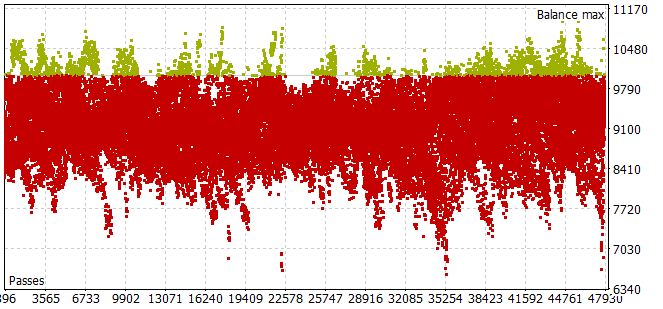
To select the optimal planning horizon in the optimization mode, the number of iterations per pass was adjusted to the optimized parameters.
After collecting the training set and training the local policy model, I ran the scheduler and cost function model training in parallel. This approach allowed me to significantly reduce the time spent training models.
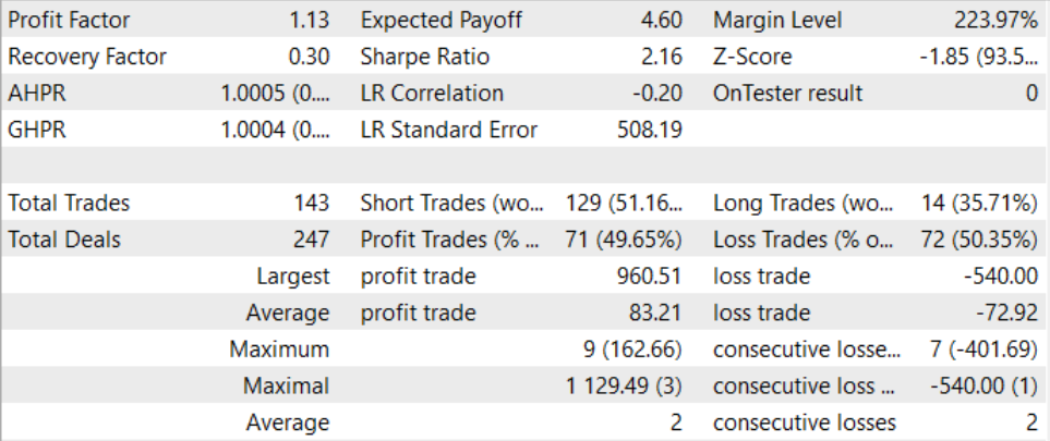
After a long and rather complex training process, we managed to obtain a model capable of generating profit outside the training set. The trained model was tested on historical data for August 2023. According to the test results, the profit factor was 1.13. The ratio of profitable and unprofitable positions is close to 1:1. All the profit is achieved due to the excess of the average profitable transaction over the average loss.
Conclusion
In this article, we introduced the Control Transformer method, which provides an innovative architecture for training control strategies in complex and dynamically changing environments. Control Transformer combines advanced reinforcement learning, scheduling and machine learning techniques to create flexible and adaptive control strategies.
Control Transformer opens up new prospects for the development of various autonomous systems and robots. Its ability to adapt to diverse environments, consider dynamic conditions and train offline makes it a powerful tool for creating intelligent and autonomous systems capable of solving complex control and navigation problems.
In the practical part of the article, we implemented our vision of the presented method using MQL5. In this implementation, we used a new approach of dividing the model training into separate unrelated EAs, which allows us to perform several tasks in parallel. This enables us to significantly reduce the overall training time of models.
While training and testing models, we managed to create a model capable of generating profit. Thus, the approach can be considered efficient. It can be used to build trading solutions.
Let me remind you once again that all the programs presented in the article are of informative nature and are intended to demonstrate the presented algorithm. They are not meant for use in real market conditions.
Links
Programs used in the article
| # | Name | Type | Description |
|---|---|---|---|
| 1 | Faza1.mq5 | Expert Advisor | Example collection EA |
| 2 | Study.mq5 | Expert Advisor | Scheduler training EA |
| 3 | StudyWorker.mq5 | Expert Advisor | Local policy model training EA |
| 4 | StudyValue.mq5 | Expert Advisor | Cost function training EA |
| 5 | Test.mq5 | Expert Advisor | Model testing EA |
| 6 | Trajectory.mqh | Class library | System state description structure |
| 7 | NeuroNet.mqh | Class library | A library of classes for creating a neural network |
| 8 | NeuroNet.cl | Code Base | OpenCL program code library |
Translated from Russian by MetaQuotes Ltd.
Original article: https://www.mql5.com/ru/articles/13674
Warning: All rights to these materials are reserved by MetaQuotes Ltd. Copying or reprinting of these materials in whole or in part is prohibited.
This article was written by a user of the site and reflects their personal views. MetaQuotes Ltd is not responsible for the accuracy of the information presented, nor for any consequences resulting from the use of the solutions, strategies or recommendations described.


- Free trading apps
- Over 8,000 signals for copying
- Economic news for exploring financial markets
You agree to website policy and terms of use