Neural networks made easy (Part 58): Decision Transformer (DT)

Introduction

In this series, we have already examined a fairly wide range of different reinforcement learning algorithms. They all use the basic approach:

1. The agent analyzes the current state of the environment.
2. Takes the optimal action (within the framework of the learned Policy - behavior strategy).
3. Moves into a new state of the environment.
4. Receives a reward from the environment for a complete transition to a new state.

The sequence is based on the principles of the Markov process. It is assumed that the starting point is the current state of the environment. There is only one optimal way out of this state and it does not depend on the previous path.

I want to introduce an alternative approach presented by the Google team in the article "Decision Transformer: Reinforcement Learning via Sequence Modeling" (06.02.2021). The main highlight of this work is the projection of the reinforcement learning problem into the modeling of a conditional sequence of actions, conditioned by an autoregressive model of the desired reward.

1. Decision Transformer method features

Decision Transformer is an architecture that changes the way we look at reinforcement learning. In contrast to the classical approach to choosing an Agent action, the problem of sequential decision making is considered within the framework of language modeling.

The method authors propose to build trajectories of the Agent’s actions in the context of previously performed actions and visited states in the same way as language models build sentences (a sequence of words) in the context of a general text. Setting the problem in this way allows the use of a wide range of language model tools with minimal modifications, including GPT (Generative Pre-trained Transformer).

It is probably worth starting with the principles of constructing the Agent’s trajectories. In this case, we are talking specifically about building trajectories, and not a sequence of actions.

One of the requirements when choosing a trajectory representation is the ability to use transformers, which will allow one to extract significant patterns in the source data. In addition to the description of environmental conditions, there will be actions and rewards performed by the Agent. The method authors offer a rather interesting approach to modeling rewards here. We want the model to generate actions based on future desired rewards, rather than past rewards. After all, our desire is to achieve some goal. Instead of delivering the reward directly, the authors provide a "Return-To-Go" magnitude model. This is analogous to a cumulative reward until the end of the episode. However, we indicate the desired result rather than the actual one.

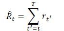
This results in the following trajectory representation, which is suitable for autoregressive learning and generation:

When testing trained models, we can specify the desired reward (for example, 1 for success or 0 for failure), as well as the initial state of the environment, as information to trigger generation. After executing the generated action for the current state, we reduce the target reward by the amount received from the environment and repeat the process until the desired total reward is received or the episode is completed.

Please note that if you use this approach and continue after reaching the desired level of total reward, a negative value may be passed to Return-To-Go. This may cause losses.

To let the agent make a decision, we pass the last K time steps to Decision Transformer as source data. In total, 3*K tokens. One for each modality: return-to-go, state and action that led to this state. To obtain vector representations of tokens, the authors of the method use a trained and fully connected neural layer for each modality, which projects the source data into the dimension of vector representations. The layer is normalized afterwards. In the case of analyzing complex (composite) environmental states, it is possible to use a convolutional encoder instead of a fully connected neural layer.

Additionally, for each time step, a vector representation of the timestamp is trained and added to each token. This approach differs from the standard positional vector representation in transformers, since one time step corresponds to several tokens (in the given example, there are three of them). The tokens are then processed using the GPT model, which predicts future action tokens using autoregressive modeling. We talked more about the architecture of GPT models when considering supervised training methods in the article "A take on GPT".

Strange as it may seem, the model training process is built using supervised learning methods. First, we arrange the interaction with the environment and sample a set of random trajectories. We have already done this multiple times. Offline training is carried out afterwards. We select mini packages of K length out of the collected set of trajectories. Prediction head corresponding to the st input token learns to predict the at action - either using the cross-entropy loss function for discrete actions, or using the mean squared error for continuous actions. The losses for each time step are averaged.

However, during the experiments, the authors of the method did not find that predicting subsequent states or rewards improved the efficiency of the models.

Below is the author's visualization of the method.

I will not dwell in detail on the architecture of transformers and the Self-Attention mechanism since these topics have already been considered before. Let's move on to the practical part and look at the implementation of the Decision Transformer mechanism using MQL5.

2. Implementation using MQL5

After a short dive into the theoretical aspects of the Decision Transformer method, let's move on to its implementation using MQL5. The first thing we are faced with is the issue of implementing embeddings of source data entities. When solving similar problems in supervised learning methods, we used convolutional layers with a step equal to the window of the original data. But in this case, there are two difficulties awaiting us:

1. The size of the environmental state description vector is different from the action space vector. The reward vector has the third size.
2. All entities contain source data from different distributions. Different embedding matrices will be required to bring them into a comparable form in a single space.

We have divided the state of the environment into two completely different blocks in content and size: historical data of price movement and a description of the current state of the account. This adds another modality for analysis. During new experiments, additional data for analysis may appear. Obviously, in such conditions we cannot use a convolutional layer and we need another universal solution capable of embedding N modalities with vector sizes [n1, n2, n3,...,nN]. As mentioned above, the method authors used trained and fully connected layers for each modality. This approach is quite universal, but in our case it entails the abandonment of parallel processing of several modalities.

In this case, the most optimal solution, in my opinion, is to create a new object in the form of a neural embedding layer CNeuronEmbeddingOCL. This is the only approach allowing us to build the process correctly. However, before creating objects and functionality of the new class, we still have to decide on some of its architectural features.

At each iteration of the forward pass, we plan to transmit five vectors of source data:

1. Historical price movement data.
2. State of an account.
3. Reward.
4. The action taken in the previous step.
5. Timestamp.

As you can see, information from different modalities differs greatly in content and volume of data. We have to determine the technology for transferring the source data to the embedding layer. Using a matrix with a separate row or column for each modality is not possible due to the different sizes of data vectors. We can, of course, use a dynamic array of vectors. But this option is only possible within the framework of implementation using MQL5. However, we will have difficulty passing such an array to the OpenCL context for parallel computing. Creating separate kernels for different numbers of source data modalities will complicate the program and will not make the algorithm completely universal. The use of one kernel for each individual modality leads to their sequential embedding and limits the possibilities of parallel computing.

In such a situation, the most universal solution, in my opinion, would be to use two vectors (buffers). In one of the vectors, we consistently indicate all the source data. In the second one, a "data map" is provided, in the form of window sizes for each sequence. Thus, using only two buffers, we can transfer any number of modalities with an independent data size to the kernel without changing the algorithm of actions inside the kernel. This is a completely universal solution with the possibility of parallel calculations for embedding all modalities at the same time.

In addition to simplicity and versatility, this approach allows us to easily combine a new class with all previously created neural layers.

We have resolved the issue with transfer of the original data. But we have almost similar situation with weight matrices. As we have already mentioned, each modality needs its own embedding matrix. However, in this case we have one advantage - the embedding sizes of all modalities are equal. After all, the goal of the embedding process is to bring different modalities to a comparable form. Therefore, each element of the source data has the same number of weighting coefficients to transfer data to the output of the neural layer. This allows us to use one common matrix to store the embedding weights of all modalities. The number of matrix columns is equal to the embedding size of one modality. The number of rows will be equal to the total number of source data. Here we can add Bayesian bias elements, which will add one row to the weight coefficient matrix for each modality.

The next constructive point that I would like to discuss is the relevance of embedding the entire preceding sequence. I do not question the need for the Agent to analyze the previous trajectory. After all, this is the basis of the method under consideration. But let's look at the issue more broadly. Decision Transformer in its essence is an autoregressive model, which receives K*N tokens as input. At each time step, only N tokens remain new. The remaining (K-1)*N tokens completely repeat the tokens used at the previous time step. Of course, at the initial stage of training, even repeated source data will have different embeddings due to changes made to the embedding matrices. But this influence will decrease as the model is trained. During everyday operation, when the weight matrices do not change, such deviations are completely absent. And it is quite logical to embed only new source data at each time step. This will allow us to significantly reduce the resource costs for data embedding during training and everyday operation of the model.

In addition, let us pay attention to one more point - positional coding. In our task, the position of historical data is indicated by the opening time of the bar. We included timestamp encoding in our source data model. But the method authors added a position token to the embedding of other modalities. This solution is fully consistent with the transformer architecture, but adds an additional operation to the sequence of actions. We will create a timestamp embedding and add it as a separate modality, because position embedding can be done in parallel with embedding of other modalities. However, this approach increases the volume of analyzed data. In each individual case, you need to take into account the balance of various factors of the program when choosing a positional encoding method.

After defining the main design features of our implementation, we can move on to building an OpenCL program. We will start, as always, by building a forward pass kernel. We want to get an embedding matrix as a result. Each row of this matrix will represent the embedding of a separate modality. Similarly, we will form a 2-dimensional space of kernel issues. In one dimension, we indicate the size of the embedding of one modality. In the second one, we indicate the number of modalities analyzed.

As you might remember, we decided to embed only the last modalities in the sequence. We transfer the embedding of the previous data without changes from the previously obtained results. At the same time, we receive the embedding of the entire sequence at the output of our CNeuronEmbeddingOCL layer.

In the kernel parameters, we pass pointers to 5 data buffers and 1 constant, in which we indicate the size of the sequence. In this case, by sequence size we mean the number of historical data steps analyzed.

In the data buffers we will pass the following information:

• inputs — initial data in the form of a sequence of all modalities (1 time step);
• outputs — sequence of embeddings of all modalities to the depth of the analyzed history;
• weights — weight ratio matrix;
• windows — source data map (sizes of data windows of each modality in the source data);
• std — vector of standard deviations (used to normalize embeddings).

__kernel void Embedding(__global float *inputs,
                        __global float *outputs,
                        __global float *weights,
                        __global int   *windows,
                        __global float *std,
                        const int stack_size
                       )
  {
   const int window_out = get_global_size(0);
   const int pos = get_local_id(0);
   const int emb = get_global_id(1);
   const int emb_total = get_global_size(1);
   const int shift_out = emb * window_out + pos;
   const int step = emb_total * window_out;
   const uint ls = min((uint)get_local_size(0), (uint)LOCAL_ARRAY_SIZE);

In the kernel body, we identify the flow in both dimensions and define offset constants in the data buffers. Then we shift the previously obtained embeddings in the results buffer. Please note that only a single embedding position is transferred in each thread. This allows arranging data copying in parallel threads.

   for(int i=stack_size-1;i>0;i--)
      outputs[i*step+shift_out]=outputs[(i-1)*step+shift_out];

The next step is to determine the offset in the source data buffer to the modality being analyzed. To do this, let’s count the total number of elements in modalities located in the source data buffer before the analyzed one.

   int shift_in = 0;
   for(int i = 0; i < emb; i++)
      shift_in += windows[i];

Here we determine the offset in the buffer of the weight matrix, taking into account the Bayesian element.

   const int shift_weights = (shift_in + emb) * window_out;

Let's save the size of the current modality's source data window into a local variable and define the constants for working with the local array.

   const int window_in = windows[emb];
   const int local_pos = (pos >= ls ? pos % (ls - 1) : pos);
   const int local_orders = (window_out + ls - 1) / ls;
   const int local_order = pos / ls;

Create a local array and fill it with zero values. Here we will set up a barrier for local thread synchronization.

   __local float temp[LOCAL_ARRAY_SIZE];
   if(local_order == 0)
      temp[local_pos] = 0;
   barrier(CLK_LOCAL_MEM_FENCE);

At this point, the preparatory work can be considered completed, and we proceed directly to embedding operations. First, we multiply the vector of input data of the analyzed modality by the corresponding vector of weight ratios. This way we get the embedding element we need.

   float value = weights[shift_weights + window_in];
   for(int i = 0; i < window_in; i++)
      value += inputs[shift_in + i] * weights[shift_weights + i];

In this case, we do not use the activation function, since we need to get the projection of each element of the sequence in the desired subspace. However, we are aware that such an approach does not guarantee the comparability of embeddings of different source data. Therefore, the next step is to normalize the data within the embedding of a single modality. Thus, we reduce the data of all embeddings to zero mean and unit variance. Let me remind you of the normalization equation.

To do this, we will first collect the sum of all elements of the analyzed embedding through a local array. Divide the resulting amount by the size of the embedding vector. This way we will determine the average value. Then we will adjust the value of the current embedding element to the average value. We use barriers to synchronize local threads.

   for(int i = 0; i < local_orders; i++)
     {
      if(i == local_order)
         temp[local_pos] += value;
      barrier(CLK_LOCAL_MEM_FENCE);
     }
//---
   int count = ls;
   do
     {
      count = (count + 1) / 2;
      if(pos < count)
         temp[pos] += temp[pos + count];
      barrier(CLK_LOCAL_MEM_FENCE);
     }
   while(count > 1);
//---
   value -= temp[0] / (float)window_out;
   barrier(CLK_LOCAL_MEM_FENCE);

Here it is worth saying a few words about the derivative of the operations performed. As you know, we use derivatives of the forward pass function to propagate the error gradient during the backward pass. When summing or subtracting a constant from a variable, we transfer the full error gradient to the variable. However, the nuance of this situation is that we are subtracting the average value. In turn, it is used as a function of the analyzed variables and has its derivative. To accurately distribute the error gradient, we need to pass it through the derivative of the mean value function. This statement is also true for the standard deviation, which we will use further. But my personal experience shows that the total error gradient passed through the derivative of the mean and variance function is several times less than the error gradient on the variable itself. In order to save resources, I will not now complicate the algorithm for storing intermediate data and subsequent calculation of error gradients in this direction.

Now let us get back to our kernel algorithm. At this stage, we have already brought the embedding vector to zero average. It is time to reduce it to unit variance. To do this, we divide all elements of the analyzed embedding by its standard deviation, which we calculate using a local array.

Let me remind you that a local array is used to transfer data between threads of a local group. Synchronization of threads is carried out through barriers.

   if(local_order == 0)
      temp[local_pos] = 0;
   barrier(CLK_LOCAL_MEM_FENCE);
//---
   for(int i = 0; i < local_orders; i++)
     {
      if(i == local_order)
         temp[local_pos] += pow(value,2.0f) / (float)window_out;
      barrier(CLK_LOCAL_MEM_FENCE);
     }
//---
   count = ls;
   do
     {
      count = (count + 1) / 2;
      if(pos < count)
         temp[pos] += temp[pos + count];
      barrier(CLK_LOCAL_MEM_FENCE);
     }
   while(count > 1);
//---
   if(temp[0] > 0)
      value /= sqrt(temp[0]);

Now we just have to save the received value into the corresponding element of the results buffer. Also do not forget to save the calculated standard deviation for the subsequent distribution of the error gradient during the reverse pass.

   outputs[shift_out] = value;
   if(pos == 0)
      std[emb] = sqrt(temp[0]);
  }

After completing work on the forward pass kernel, I propose to move on to analyzing the error gradient distribution kernel algorithm. We have already started discussing the distribution of the error gradient through the data normalization function above. To optimize the use of resources, it was decided to simplify the algorithm in terms of the error gradient through the functions of the average value and dispersion of the embedding vector. At this stage, we treat the mean and variance as constants. It is in this paradigm that the EmbeddingHiddenGradient error gradient kernel algorithm is built.

In the kernel parameters, we pass 5 data buffers and 1 constant. We have already become familiar with the constant and 3 of the buffers used in the previous kernel. The buffers of the original data and results are replaced with buffers of the corresponding error gradients.

__kernel void EmbeddingHiddenGradient(__global float *inputs_gradient,
                                      __global float *outputs_gradient,
                                      __global float *weights,
                                      __global int   *windows,
                                      __global float *std,
                                      const int window_out
                                     )
  {
   const int pos = get_global_id(0);

We will call the kernel in a one-dimensional task space according to the number of elements of the source data. In the body of the kernel, we immediately identify the current thread. However, the position of an element in the source data buffer does not give us an explicit idea of the dependent elements in the result buffer. Therefore, we first iterate through the raw data map buffer to determine the modality to be analyzed.

   int emb = -1;
   int count = 0;
   do
     {
      emb++;
      count += windows[emb];
     }
   while(count <= pos);

 Based on the index of the modality being analyzed, we determine the bias in the result and weight buffers.

   const int shift_out = emb * window_out;
   const int shift_weights = (pos + emb) * window_out;

After determining the biases in the data buffers, we collect error gradients from all dependent elements of the result buffer and adjust them by the standard deviation of the embedding vector before normalization. Let me remind you that we saved its value in the std buffer during the direct passage.

   float value = 0;
   for(int i = 0; i < window_out; i++)
      value += outputs_gradient[shift_out + i] * weights[shift_weights + i];
   float s = std[emb];
   if(s > 0)
      value /= s;
//---
   inputs_gradient[pos] = value;
  }

The resulting value is stored in the gradient buffer of the previous layer.

To complete the work with the OpenCL program, we just need to consider the kernel algorithm for updating the weight matrix. In this article, we will only look at the kernel of the Adam method, which I use most often. The main difference between this kernel and similar ones discussed earlier lies in the determination of offsets in data buffers. This is quite expected. We are not making fundamental changes to the algorithm of the weight ratios updating method itself.

__kernel void EmbeddingUpdateWeightsAdam(__global float *weights,
                                          __global const float *gradient,
                                          __global const float *inputs,   
                                          __global float *matrix_m,       
                                          __global float *matrix_v,       
                                          __global int   *windows,
                                          __global float *std,
                                          const int window_out,
                                          const float l,                  
                                          const float b1,               
                                          const float b2                
                                        )
  {
   const int i = get_global_id(0);

A fairly large number of buffers and constants are passed in the kernel parameters. We already know all of them. The kernel will be called in a one-dimensional task space based on the number of elements in the weight ratio buffer.

In the kernel body, we, as usual, identify the buffer element being analyzed by the thread ID. After that, we determine the offsets in the data buffers to the elements we need.

   int emb = -1;
   int count = 0;
   int shift = 0;
   do
     {
      emb++;
      shift = count;
      count += (windows[emb] + 1) * window_out;
     }
   while(count <= i);
   const int shift_out = emb * window_out;
   int shift_in = shift / window_out - emb;
   shift = (i - shift) / window_out;

Then we arrange adjustments to the weighting ratio. The process completely repeats the one discussed in previous articles of the series. Save the result and the necessary data into the appropriate buffers.

   float weight = weights[i];
   float g = gradient[shift_out] * inp / std[emb];
   float mt = b1 * matrix_m[i] + (1 - b1) * g;
   float vt = b2 * matrix_v[i] + (1 - b2) * pow(g, 2);
   float delta = l * (mt / (sqrt(vt) + 1.0e-37f) - (l1 * sign(weight) + l2 * weight));
   if(delta * g > 0)
      weights[i] = clamp(weights[i] + delta, -MAX_WEIGHT, MAX_WEIGHT);
   matrix_m[i] = mt;
   matrix_v[i] = vt;
  }

After finishing work on the kernels of the OpenCL program, we return to work on the side of the main program. Now that we already have clarity of the class functionality and a complete list of necessary data buffers, we can create all the conditions for calling and maintaining the kernels discussed above.

As mentioned above, we create a new class CNeuronEmbeddingOCL based on the CNeuronBaseOCL base class of neural layers. The main functionality of the neural layer is inherited from the parent class. We have to add new functionality to the class.

Create the a_Windows dynamic array to store the source data map. However, we will not create a separate buffer object to maintain it. Instead, let's create a variable to record a pointer to the buffer in the i_WindowsBuffer OpenCL context. Here we will create variables to record the size of one embedding and the depth of the analyzed history — i_WindowOut and i_StackSize, respectively.

Create data buffers for the matrix of embedding weight ratios and moments:

• WeightsEmbedding;
• FirstMomentumEmbed;
• SecondMomentumEmbed.

But the standard deviation buffer is used only for intermediate calculations. Therefore, we will not create it on the side of the main program. Let's create it only in the OpenCL context memory and store a pointer to it in the i_STDBuffer variable.

The set of overridden methods is quite standard and we will not dwell on their purpose now.

class CNeuronEmbeddingOCL  :  public CNeuronBaseOCL
  {
protected:
   int               a_Windows[];
   int               i_WindowOut;
   int               i_StackSize;
   int               i_WindowsBuffer;
   int               i_STDBuffer;
   //---
   CBufferFloat      WeightsEmbedding;
   CBufferFloat      FirstMomentumEmbed;
   CBufferFloat      SecondMomentumEmbed;

   virtual bool      feedForward(CNeuronBaseOCL *NeuronOCL);               
   virtual bool      updateInputWeights(CNeuronBaseOCL *NeuronOCL); 

public:
                     CNeuronEmbeddingOCL(void);
                    ~CNeuronEmbeddingOCL(void);
   //---
   virtual bool      Init(uint numOutputs, uint myIndex, COpenCLMy *open_cl, uint stack_size, uint window_out, int &windows[]);
   //---
   virtual bool      calcInputGradients(CNeuronBaseOCL *NeuronOCL);          
   //---
   virtual bool      Save(int const file_handle);
   virtual bool      Load(int const file_handle);
   //---
   virtual int       Type(void)        const                      {  return defNeuronEmbeddingOCL;                  }
   virtual CLayerDescription* GetLayerInfo(void);
   virtual void      SetOpenCL(COpenCLMy *obj);
   virtual bool      Clear(void);
  };

In the class constructor, initialize variables and pointers to buffers with initial values.

CNeuronEmbeddingOCL::CNeuronEmbeddingOCL(void)
  {
   ArrayFree(a_Windows);
   if(!!OpenCL)
     {
      if(i_WindowsBuffer >= 0)
         OpenCL.BufferFree(i_WindowsBuffer);
      if(i_STDBuffer >= 0)
         OpenCL.BufferFree(i_STDBuffer);
     }
//--
   i_WindowsBuffer = INVALID_HANDLE;
   i_STDBuffer = INVALID_HANDLE;
   i_WindowOut = 0;
   i_StackSize = 1;
  }

Direct initialization of the embedding layer object is carried out in the Init method. In addition to the constants, we convey the depth of the analyzed history (stack_size), embedding vector size (window_out) and "source data map" (windows[] dynamic array) in the method parameters.

bool CNeuronEmbeddingOCL::Init(uint numOutputs,uint myIndex,COpenCLMy *open_cl,uint stack_size, uint window_out,int &windows[])
  {
   if(CheckPointer(open_cl) == POINTER_INVALID || window_out <= 0 || windows.Size() <= 0 || stack_size <= 0)
      return false;
   if(!!OpenCL && OpenCL != open_cl)
      delete OpenCL;
   uint numNeurons = window_out * windows.Size() * stack_size;
   if(!CNeuronBaseOCL::Init(numOutputs,myIndex,open_cl,numNeurons,ADAM,1))
      return false;

We create a source data control block in the method body. Then we recalculate the size of the results buffer as the product of the length of the vector of one embedding by the number of modalities and the depth of the analyzed history. Note that there is no total number of modalities in the external parameters. But we get the "map of initial data". The size of the resulting array will tell us the number of modalities being analyzed.

Direct initialization of the results buffer, as well as other inherited objects, is carried out in a similar method of the parent class, which we call after completing the preparatory operations.

After successful initialization of the inherited objects, we need to prepare the added entities. First, we initialize the embedding weight buffer. As described above, this buffer is a matrix with a number of rows equal to the volume of the original data and columns equal to the size of the vector of one embedding. We know the size of the embedding. But to determine the size of the source data, we need to sum up all the values of the "data map". Add one line of Bayesian bias to the resulting sum for each modality. This way we get the size of the embedding weight buffer. Now we will fill it with random values and transfer it to OpenCL context memory.

   uint weights = 0;
   ArrayCopy(a_Windows,windows);
   i_WindowOut = (int)window_out;
   i_StackSize = (int)stack_size;
   for(uint i = 0; i < windows.Size(); i++)
      weights += (windows[i] + 1) * window_out;
   if(!WeightsEmbedding.Reserve(weights))
      return false;
   float k = 1.0f / sqrt((float)weights / (float)window_out);
   for(uint i = 0; i < weights; i++)
      if(!WeightsEmbedding.Add(k * (2 * GenerateWeight() - 1.0f)*WeightsMultiplier))
         return false;
   if(!WeightsEmbedding.BufferCreate(OpenCL))
      return false;

The first and second moment buffers are of similar size. But we initialize them with zero values and transfer them to the OpenCL context memory.

   if(!FirstMomentumEmbed.BufferInit(weights, 0))
      return false;
   if(!FirstMomentumEmbed.BufferCreate(OpenCL))
      return false;
//---
   if(!SecondMomentumEmbed.BufferInit(weights, 0))
      return false;
   if(!SecondMomentumEmbed.BufferCreate(OpenCL))
      return false;

Next, we create the raw data and standard deviation map buffers.

   i_WindowsBuffer = OpenCL.AddBuffer(sizeof(int) * a_Windows.Size(),CL_MEM_READ_WRITE);
   if(i_WindowsBuffer < 0 || !OpenCL.BufferWrite(i_WindowsBuffer,a_Windows,0,0,a_Windows.Size()))
      return false;
   i_STDBuffer = OpenCL.AddBuffer(sizeof(float) * a_Windows.Size(),CL_MEM_READ_WRITE);
   if(i_STDBuffer<0)
     return false;
//---
   return true;
  }

We make sure to control the process of performing operations at each step. After completing all operations of the method, return the logical result of the method to the calling program.

After initializing the object, we have to create methods for its main functionality. In our case, these are forward and backward pass methods. As you may have guessed, we have already done the main work on arranging the functionality in the OpenCL program. Now all we have to do is organize the call of the appropriate kernels. Before starting, we need to declare constants for working with kernels: kernel IDs in the program and their parameters. As always, we perform this functionality using the #define directive.

#define def_k_Embedding                59
#define def_k_emb_inputs               0
#define def_k_emb_outputs              1
#define def_k_emb_weights              2
#define def_k_emb_windows              3
#define def_k_emb_std                  4
#define def_k_emb_stack_size           5
//---
#define def_k_EmbeddingHiddenGradient  60
#define def_k_ehg_inputs_gradient      0
#define def_k_ehg_outputs_gradient     1
#define def_k_ehg_weights              2
#define def_k_ehg_windows              3
#define def_k_ehg_std                  4
#define def_k_ehg_window_out           5
//---
#define def_k_EmbeddingUpdateWeightsAdam  61
#define def_k_euw_weights              0
#define def_k_euw_gradient             1
#define def_k_euw_inputs               2
#define def_k_euw_matrix_m             3
#define def_k_euw_matrix_v             4
#define def_k_euw_windows              5
#define def_k_euw_std                  6
#define def_k_euw_window_out           7
#define def_k_euw_learning_rate        8
#define def_k_euw_b1                   9
#define def_k_euw_b2                   10

We will look at arranging the process of placing the kernel into the execution queue using the example of the feedForward direct pass method. In the method parameters, as in all similar ones previously considered, we receive the pointer to the object of the previous neural layer.

bool CNeuronEmbeddingOCL::feedForward(CNeuronBaseOCL *NeuronOCL)
  {
   if(!NeuronOCL || !OpenCL)
      return false;

In the method body, we check the received pointer and the pointer to the object for working with the OpenCL context.

Next, we pass pointers to the data buffers and the necessary constants that were previously specified in the kernel parameters to the kernel. Do not forget to monitor operations at every step.

   if(!OpenCL.SetArgumentBuffer(def_k_Embedding, def_k_emb_inputs, NeuronOCL.getOutputIndex()))
     {
      printf("Error of set parameter kernel %s: %d; line %d", __FUNCTION__,GetLastError(), __LINE__);
      return false;
     }
   if(!OpenCL.SetArgumentBuffer(def_k_Embedding, def_k_emb_outputs, getOutputIndex()))
     {
      printf("Error of set parameter kernel %s: %d; line %d", __FUNCTION__,GetLastError(), __LINE__);
      return false;
     }
   if(!OpenCL.SetArgumentBuffer(def_k_Embedding, def_k_emb_std, i_STDBuffer))
     {
      printf("Error of set parameter kernel %s: %d; line %d", __FUNCTION__,GetLastError(), __LINE__);
      return false;
     }
   if(!OpenCL.SetArgumentBuffer(def_k_Embedding, def_k_emb_weights, WeightsEmbedding.GetIndex()))
     {
      printf("Error of set parameter kernel %s: %d; line %d", __FUNCTION__,GetLastError(), __LINE__);
      return false;
     }
   if(!OpenCL.SetArgumentBuffer(def_k_Embedding, def_k_emb_windows, i_WindowsBuffer))
     {
      printf("Error of set parameter kernel %s: %d; line %d", __FUNCTION__,GetLastError(), __LINE__);
      return false;
     }
   if(!OpenCL.SetArgument(def_k_Embedding, def_k_emb_stack_size, i_StackSize))
     {
      printf("Error of set parameter kernel %s: %d; line %d", __FUNCTION__,GetLastError(), __LINE__);
      return false;
     }

After successfully passing all the parameters, we need to define the task space for the kernel. As we discussed above, the kernel will run in a 2-dimensional task space. In the first dimension, we will indicate the size of one embedding, while in the second, we specify the number of modalities for analysis.

   uint global_work_offset[2] = {0,0};
   uint global_work_size[2]   = {i_WindowOut,a_Windows.Size()};

A feature of the embedding kernel is the normalization of data within the embedding vector of one modality. To build this subprocess, we organized data exchange between threads within the same workgroup through a local array. Now we need to specify the size of the local group, which is equal to the size of the embedding vector. The nuance is that when specifying a 2-dimensional space, we need to specify a 2-dimensional local group. Therefore the 2nd dimension of the local group is 1.

   uint local_work_size[2]    = {i_WindowOut,1};

Finally, call the method for queuing the kernel and control the process of performing operations.

   if(!OpenCL.Execute(def_k_Embedding, 2, global_work_offset, global_work_size,local_work_size))
     {
      printf("Error of execution kernel %s: %d", __FUNCTION__,GetLastError());
      return false;
     }
//---
   return true;
  }

The procedure for calling backpass kernels is similar, and we will not dwell on these methods now. You can find all necessary code in the attachment. I would like to focus on the following point. Decision Transformer is an autoregressive model and the consistency of the input data is of great importance. Above, we determined that at each time step we feed only new data to the model input. The entire depth of the analyzed history is copied from previous model operations. Essentially, we use the CNeuronEmbeddingOCL layer's result buffer as an embedding stack. This approach allows reducing the costs of primary data processing. However, it introduces a requirement for the consistent supply of initial data both during the training process and during operation. At the same time, we often use random samples of source data during training. The need for this has been discussed more than once before. In order to exclude data corruption as a result of a "temporary jump" in the original data or when switching to an alternative trajectory, we need a method for clearing the embedding stack. The Clear method was created for these purposes. Its algorithm is quite simple: we just fill the entire buffer with zero values and copy the data into the OpenCL context memory.

bool CNeuronEmbeddingOCL::Clear(void)
  {
   if(!Output.BufferInit(Output.Total(),0))
      return false;
   if(!OpenCL)
      return true;
//---
   return Output.BufferWrite();
  }

This concludes the discussion of the CNeuronEmbeddingOCL class method algorithms. You can find its full code and all methods in the attachment.

As a result of the work done, we have comparable embeddings of several different modalities at the output of the CNeuronEmbeddingOCL layer. This allows us to use previously created transformer objects to implement the presented Decision Transformer method. This means we can move on to working on a description of the model architecture. In this case we will use only one model - the Agent one. It's been a while since this happened in our series of articles.

But first, I must remind you of the "source map". To describe it, we used an array that was not previously in the neural layer description class. Let's add it.

class CLayerDescription    :  public CObject
  {
public:
   /** Constructor */
                     CLayerDescription(void);
   /** Destructor */~CLayerDescription(void) {};
   //---
   int               type;          ///< Type of neurons in layer (\ref ObjectTypes)
   int               count;         ///< Number of neurons
   int               window;        ///< Size of input window
   int               window_out;    ///< Size of output window
   int               step;          ///< Step size
   int               layers;        ///< Layers count
   int               batch;         ///< Batch Size
   ENUM_ACTIVATION   activation;    ///< Type of activation function (#ENUM_ACTIVATION)
   ENUM_OPTIMIZATION optimization;  ///< Type of optimization method (#ENUM_OPTIMIZATION)
   float             probability;   ///< Probability of neurons shutdown, only Dropout used
   int               windows[];
   //---
   virtual bool      Copy(CLayerDescription *source);
   //---
   virtual bool      operator= (CLayerDescription *source)  { return Copy(source); }
  };

We describe the model architecture in the CreateDescriptions method. In the parameters, the method receives a pointer to only one dynamic array describing the Actor's architecture. We will save the description of the neural layers of the model into the resulting array.

bool CreateDescriptions(CArrayObj *agent)
  {
//---
   CLayerDescription *descr;
//---
   if(!agent)
     {
      agent = new CArrayObj();
      if(!agent)
         return false;
     }
//--- Agent
   agent.Clear();

As the first layer, we will indicate a fully connected neural layer of the source data, into which we will sequentially write all the data necessary for analysis. Please note that we do not split the source data into separate buffers based on content. In this case, their division is rather arbitrary. We just write them down sequentially. Their logical separation will be carried out at the embedding level according to the "source data map", which we will create later.

Note that the source data layer only contains information about the last state of the system (reward, environmental state, account state, timestamp and last Agent action).

//--- Input layer
   if(!(descr = new CLayerDescription()))
      return false;
   descr.type = defNeuronBaseOCL;
   int prev_count = descr.count = (NRewards + BarDescr*NBarInPattern + AccountDescr + TimeDescription + NActions);
   descr.activation = None;
   descr.optimization = ADAM;
   if(!agent.Add(descr))
     {
      delete descr;
      return false;
     }

Following the source data layer, we will indicate the batch normalization layer, in which data preprocessing is carried out. Again, we do not think about the different nature of the data obtained. After all, this layer carries out normalization in the context of historical data for each attribute independently.

//--- layer 1
   if(!(descr = new CLayerDescription()))
      return false;
   descr.type = defNeuronBatchNormOCL;
   descr.count = prev_count;
   descr.batch = 1000;
   descr.activation = None;
   descr.optimization = ADAM;
   if(!agent.Add(descr))
     {
      delete descr;
      return false;
     }

Next comes the batch normalization layer. Here we indicate the depth of the analyzed history, the size of the vector of one embedding and the "source data map".

//--- layer 2
   if(!(descr = new CLayerDescription()))
      return false;
   descr.type = defNeuronEmbeddingOCL;
   prev_count = descr.count = HistoryBars;
     {
      int temp[] = {BarDescr*NBarInPattern,AccountDescr,TimeDescription,NRewards,NActions};
      ArrayCopy(descr.windows,temp);
     }
   int prev_wout = descr.window_out = EmbeddingSize;
   if(!agent.Add(descr))
     {
      delete descr;
      return false;
     }

Behind the embedding layer, we will place a sparse attention block defNeuronMLMHSparseAttentionOCL, which will form the basis of our transformer. The method authors used an original transformer. However, using a sparse attention block will allow us to significantly increase the depth of the analyzed history with a slight increase in resource costs and model running time.

//--- layer 3
   if(!(descr = new CLayerDescription()))
      return false;
   descr.type = defNeuronMLMHSparseAttentionOCL;
   descr.count = prev_count;
   descr.window = prev_wout;
   descr.step = 4;
   descr.window_out = 16;
   descr.layers = 4;
   descr.probability = Sparse;
   descr.optimization = ADAM;
   if(!agent.Add(descr))
     {
      delete descr;
      return false;
     }

The model is completed with a decision-making block of fully connected layers and a latent layer of a variational autoencoder at the output to create stochasticity in the Actor’s policy.

//--- layer 4
   if(!(descr = new CLayerDescription()))
      return false;
   descr.type = defNeuronBaseOCL;
   descr.count = LatentCount;
   descr.optimization = ADAM;
   descr.activation = LReLU;
   if(!agent.Add(descr))
     {
      delete descr;
      return false;
     }
//--- layer 5
   if(!(descr = new CLayerDescription()))
      return false;
   descr.type = defNeuronBaseOCL;
   prev_count = descr.count = LatentCount;
   descr.activation = TANH;
   descr.optimization = ADAM;
   if(!agent.Add(descr))
     {
      delete descr;
      return false;
     }
//--- layer 6
   if(!(descr = new CLayerDescription()))
      return false;
   descr.type = defNeuronBaseOCL;
   descr.count = LatentCount;
   descr.activation = LReLU;
   descr.optimization = ADAM;
   if(!agent.Add(descr))
     {
      delete descr;
      return false;
     }
//--- layer 7
   if(!(descr = new CLayerDescription()))
      return false;
   descr.type = defNeuronBaseOCL;
   descr.count = 2 * NActions;
   descr.activation = SIGMOID;
   descr.optimization = ADAM;
   if(!agent.Add(descr))
     {
      delete descr;
      return false;
     }
//--- layer 8
   if(!(descr = new CLayerDescription()))
      return false;
   descr.type = defNeuronVAEOCL;
   descr.count = NActions;
   descr.optimization = ADAM;
   if(!agent.Add(descr))
     {
      delete descr;
      return false;
     }
//---
   return true;
  }

It must be said that the decision-making block also differs from that used in the author’s DT algorithm. The method authors used the decoder of the last token in the sequence at the output of the transformer. We analyze the entire sequence to make an informed decision.

After specifying the model architecture, we proceed to creating an EA for interacting with the environment and collecting data for training the model into the experience playback buffer "\DT\Research.mq5". The EA structure is completely the same as the ones discussed earlier, but it is worth focusing on the OnTick tick processing method. It is here that the sequence of initial data is formed in accordance with the map described above.

In the method body, we check for the occurrence of the event of opening a new bar and, if necessary, load historical data. However, now we are not loading the entire depth of the analyzed history, but only updates in the size of the pattern of one time step. This can be data from one last closed candle or maybe more. We introduced the NBarInPattern constant to regulate the depth of data loading. Please do not confuse it with the HistoryBars constant, which we will use to determine the depth of the embedding stack.

void OnTick()
  {
//---
   if(!IsNewBar())
      return;
//---
   int bars = CopyRates(Symb.Name(), TimeFrame, iTime(Symb.Name(), TimeFrame, 1), NBarInPattern, Rates);
   if(!ArraySetAsSeries(Rates, true))
      return;
//---
   RSI.Refresh();
   CCI.Refresh();
   ATR.Refresh();
   MACD.Refresh();
   Symb.Refresh();
   Symb.RefreshRates();

Then we create an array from the historical data to store in the trajectory and transfer it to the source data buffer. The procedure is completely identical to the previously discussed EAs.

//--- History data
   float atr = 0;
   for(int b = 0; b < (int)NBarInPattern; b++)
     {
      float open = (float)Rates[b].open;
      float rsi = (float)RSI.Main(b);
      float cci = (float)CCI.Main(b);
      atr = (float)ATR.Main(b);
      float macd = (float)MACD.Main(b);
      float sign = (float)MACD.Signal(b);
      if(rsi == EMPTY_VALUE || cci == EMPTY_VALUE || atr == EMPTY_VALUE || macd == EMPTY_VALUE || sign == EMPTY_VALUE)
         continue;
      //---
      int shift = b * BarDescr;
      sState.state[shift] = (float)(Rates[b].close - open);
      sState.state[shift + 1] = (float)(Rates[b].high - open);
      sState.state[shift + 2] = (float)(Rates[b].low - open);
      sState.state[shift + 3] = (float)(Rates[b].tick_volume / 1000.0f);
      sState.state[shift + 4] = rsi;
      sState.state[shift + 5] = cci;
      sState.state[shift + 6] = atr;
      sState.state[shift + 7] = macd;
      sState.state[shift + 8] = sign;
     }
   bState.AssignArray(sState.state);

The next step is to create a description of the account status. Data collection is carried out according to a previously applied procedure. However, the data is transferred not to a separate buffer, but to the bState single original data buffer.

//--- Account description
   sState.account[0] = (float)AccountInfoDouble(ACCOUNT_BALANCE);
   sState.account[1] = (float)AccountInfoDouble(ACCOUNT_EQUITY);
//---
   double buy_value = 0, sell_value = 0, buy_profit = 0, sell_profit = 0;
   double position_discount = 0;
   double multiplyer = 1.0 / (60.0 * 60.0 * 10.0);
   int total = PositionsTotal();
   datetime current = TimeCurrent();
   for(int i = 0; i < total; i++)
     {
      if(PositionGetSymbol(i) != Symb.Name())
         continue;
      double profit = PositionGetDouble(POSITION_PROFIT);
      switch((int)PositionGetInteger(POSITION_TYPE))
        {
         case POSITION_TYPE_BUY:
            buy_value += PositionGetDouble(POSITION_VOLUME);
            buy_profit += profit;
            break;
         case POSITION_TYPE_SELL:
            sell_value += PositionGetDouble(POSITION_VOLUME);
            sell_profit += profit;
            break;
        }
      position_discount += profit - (current - PositionGetInteger(POSITION_TIME)) * multiplyer * MathAbs(profit);
     }
   sState.account[2] = (float)buy_value;
   sState.account[3] = (float)sell_value;
   sState.account[4] = (float)buy_profit;
   sState.account[5] = (float)sell_profit;
   sState.account[6] = (float)position_discount;
   sState.account[7] = (float)Rates[0].time;
//---
   bState.Add((float)((sState.account[0] - PrevBalance) / PrevBalance));
   bState.Add((float)(sState.account[1] / PrevBalance));
   bState.Add((float)((sState.account[1] - PrevEquity) / PrevEquity));
   bState.Add(sState.account[2]);
   bState.Add(sState.account[3]);
   bState.Add((float)(sState.account[4] / PrevBalance));
   bState.Add((float)(sState.account[5] / PrevBalance));
   bState.Add((float)(sState.account[6] / PrevBalance));

Add the timestamp to the same buffer.

//--- Time label
   double x = (double)Rates[0].time / (double)(D'2024.01.01' - D'2023.01.01');
   bState.Add((float)MathSin(2.0 * M_PI * x));
   x = (double)Rates[0].time / (double)PeriodSeconds(PERIOD_MN1);
   bState.Add((float)MathCos(2.0 * M_PI * x));
   x = (double)Rates[0].time / (double)PeriodSeconds(PERIOD_W1);
   bState.Add((float)MathSin(2.0 * M_PI * x));
   x = (double)Rates[0].time / (double)PeriodSeconds(PERIOD_D1);
   bState.Add((float)MathSin(2.0 * M_PI * x));

The following data is already generated by the requirements of the Decision Transformer method. Here we add the Return-To-Go modality to the source data buffer. There may be one element of the desired reward or a vector of decomposed rewards. We will indicate 3 elements: balance change, equity change and drawdown. All 3 indicators are indicated in relative values.

//--- Return to go
   bState.Add(float(1-(sState.account[0] - PrevBalance) / PrevBalance));
   bState.Add(float(0.1f-(sState.account[1] - PrevEquity) / PrevEquity));
   bState.Add(0);

To complete the vector of initial data, we add the vector of the Agent’s latest actions. When called for the first time, this vector is filled with zero values.

//--- Prev action
   bState.AddArray(AgentResult);

The source data vector is ready, and we perform a direct pass of the Agent.

   if(!Agent.feedForward(GetPointer(bState), 1, false, (CBufferFloat*)NULL))
      return;

The further algorithm for interpreting the model results and making transactions has been transferred without changes, and we will not dwell on it. You can find the full code of the EA and all its methods in the attachment. Let's move on to building the model training process in the "\DT\Study.mq5" EA. The EA also inherited a lot from previous works. Now we will dwell in detail only on the Train model training method.

In the method body, we first determine the number of trajectories stored in the local experience replay buffer.

void Train(void)
  {
   int total_tr = ArraySize(Buffer);
   uint ticks = GetTickCount();

Then we arrange a cycle based on the number of training iterations, in which we randomly select one trajectory and a separate state on this trajectory. Everything here is the same as before.

   bool StopFlag = false;
   for(int iter = 0; (iter < Iterations && !IsStopped() && !StopFlag); iter ++)
     {
      int tr = (int)((MathRand() / 32767.0) * (total_tr - 1));
      int i = (int)((MathRand() * MathRand() / MathPow(32767, 2)) * MathMax(Buffer[tr].Total - 2 * HistoryBars,MathMin(Buffer[tr].Total,20)));
      if(i < 0)
        {
         iter--;
         continue;
        }

Here is where the differences start. Remember that we talked about the need to supply sequential data to the input of the model. But we are a random state on a trajectory. In order to eliminate data corruption in the analyzed sequence, we clear the embedding buffer and the vector of the Agent’s last actions.

      Actions = vector<float>::Zeros(NActions);
      Agent.Clear();

Then we organize a nested loop, the number of iterations of which is 3 times the depth of the analyzed history, of course, if the size of the saved trajectory allows doing that. In the body of this nested loop, we will train the model by feeding it input data from the saved trajectory in a strict sequence of interaction with the environment. First, we will load historical indicator price movement data into the buffer.

      for(int state = i; state < MathMin(Buffer[tr].Total - 1,i + HistoryBars * 3); state++)
        {
         //--- History data
         State.AssignArray(Buffer[tr].States[state].state);

The following is information about the account status.

         //--- Account description
         float PrevBalance = (state == 0 ? Buffer[tr].States[state].account[0] : Buffer[tr].States[state - 1].account[0]);
         float PrevEquity = (state == 0 ? Buffer[tr].States[state].account[1] : Buffer[tr].States[state - 1].account[1]);
         State.Add((Buffer[tr].States[state].account[0] - PrevBalance) / PrevBalance);
         State.Add(Buffer[tr].States[state].account[1] / PrevBalance);
         State.Add((Buffer[tr].States[state].account[1] - PrevEquity) / PrevEquity);
         State.Add(Buffer[tr].States[state].account[2]);
         State.Add(Buffer[tr].States[state].account[3]);
         State.Add(Buffer[tr].States[state].account[4] / PrevBalance);
         State.Add(Buffer[tr].States[state].account[5] / PrevBalance);
         State.Add(Buffer[tr].States[state].account[6] / PrevBalance);

And a timestamp.

         //--- Time label
         double x = (double)Buffer[tr].States[state].account[7] / (double)(D'2024.01.01' - D'2023.01.01');
         State.Add((float)MathSin(2.0 * M_PI * x));
         x = (double)Buffer[tr].States[state].account[7] / (double)PeriodSeconds(PERIOD_MN1);
         State.Add((float)MathCos(2.0 * M_PI * x));
         x = (double)Buffer[tr].States[state].account[7] / (double)PeriodSeconds(PERIOD_W1);
         State.Add((float)MathSin(2.0 * M_PI * x));
         x = (double)Buffer[tr].States[state].account[7] / (double)PeriodSeconds(PERIOD_D1);
         State.Add((float)MathSin(2.0 * M_PI * x));

At this stage, we transfer the actual accumulative reward to the end of the trajectory in Return-To-Go. The approach is slightly different from a similar token in the environment interaction EA. But this is what allows us to train the model.

         //--- Return to go
         State.AddArray(Buffer[tr].States[state].rewards);

Add the Agent’s action at the previous time step from the experience playback buffer.

         //--- Prev action
         State.AddArray(Actions);

The source data buffer for one training iteration is ready, and we call the Agent's forward pass method.

         //--- Feed Forward
         if(!Agent.feedForward(GetPointer(State), 1, false, (CBufferFloat*)NULL))
           {
            PrintFormat("%s -> %d", __FUNCTION__, __LINE__);
            StopFlag = true;
            break;
           }

After successfully completing the forward pass, we have to perform a reverse pass and adjust the model parameters. Here the question of target values arises, which is solved in a quite simple manner. We use the actions actually performed by the Agent when interacting with the environment as target values. Paradoxically, this is a pure supervised training. But where is reinforcement learning? Where are the reward optimizations? We cannot even use supervised learning because actions taken when interacting with the environment are not optimal.

We train an autoregressive model, which, based on knowledge of the trajectory traveled and the desired result, generates an optimal action. In this aspect, the main role is played by indicating the actual accumulated reward in the return-to-go token. After all, no one doubts that it was the actions actually performed that led to the actual rewards received. Therefore, we can easily train the model to identify these actions with the reward received. A well-trained model will subsequently be able to generate actions to obtain the desired result during operation.

Decision Transformer authors suggest using MSE for a continuous action space. We will supplement it with the CAGrad method.

         //--- Policy study
         Actions.Assign(Buffer[tr].States[state].action);
         vector<float> result;
         Agent.getResults(result);
         Result.AssignArray(CAGrad(Actions - result) + result);
         if(!Agent.backProp(Result, (CBufferFloat*)NULL))
           {
            PrintFormat("%s -> %d", __FUNCTION__, __LINE__);
            StopFlag = true;
            break;
           }

After a successful reverse pass, we inform the user about the state of training and move on to the next iteration of our learning process loop system. Upon completion of all iterations, we initiate the process of terminating the EA work.

   Comment("");
//---
   PrintFormat("%s -> %d -> %-15s %10.7f", __FUNCTION__, __LINE__, "Agent", Agent.getRecentAverageError());
   ExpertRemove();
//---
  }

Find the complete code of all programs used in the article in the attachment.

3. Test

We have done quite a lot of work to implement the Decision Transformer method using MQL5. It is time to train and test the model. As always, training and testing of models is carried out on EURUSD H1. The parameters of all indicators are used by default. The training period is 7 months of 2023. We will test the model using historical data for August 2023.

Based on the results of testing this method, we can say that the idea is quite interesting. But in a stochastic market, I managed to achieve the desired result. While it is still possible to achieve acceptable results on the training sample, we see an increase in the balance in the first ten days of the testing period on the new data. But then comes a series of losing trades. As a result, the model produced losses on test data. Although we see the average winning trade exceeding the average loss by a little more than 1.0%, this is not enough. The share of profitable transactions is only 47.76%. The bottom line is the profit factor of 0.92.

Conclusion

In this article, I introduced a rather interesting method called Decision Transformer, which is a new and innovative approach to reinforcement learning. Unlike traditional methods, Decision Transformer models action sequences in the context of an autoregressive model of desired rewards. This allows the Agent to learn to make decisions based on future goals and optimize its behavior based on these goals.

In the practical part of the article, we implemented the presented method using MQL5, conducted training and testing of the model. However, the trained model was unable to generate profits throughout the test period. In the first half of the test sample, the model made a profit, but all of it was lost when testing continued. The algorithm has potential. However, additional work with the model is necessary to obtain the desired results.

Links

• Decision Transformer: Reinforcement Learning via Sequence Modeling
• Neural networks made easy (Part 57): Stochastic Marginal Actor-Critic (SMAC)

Programs used in the article

#	Name	Type	Description
1	Research.mq5	Expert Advisor	Example collection EA
2	Study.mq5	Expert Advisor	Agent training EA
3	Test.mq5	Expert Advisor	Model testing EA
4	Trajectory.mqh	Class library	System state description structure
5	NeuroNet.mqh	Class library	A library of classes for creating a neural network
6	NeuroNet.cl	Code Base	OpenCL program code library