
Neural networks made easy (Part 61): Optimism issue in offline reinforcement learning

Introduction
Recently, offline reinforcement learning methods have become widespread, which promises many prospects in solving problems of varying complexity. However, one of the main problems that researchers face is the optimism that can arise while learning. The agent optimizes its strategy based on the data from the training set and gains confidence in its actions. But the training set is quite often not able to cover the entire variety of possible states and transitions of the environment. In a stochastic environment, such confidence turns out to be not entirely justified. In such cases, the agent's optimistic strategy may lead to increased risks and undesirable consequences.
In search of a solution to this problem, it is worth paying attention to research in the field of autonomous driving. It is obvious that the algorithms in this area are aimed at reducing risks (increasing user safety) and minimizing online training. One such method is SeParated Latent Trajectory Transformer (SPLT-Transformer) presented in the article "Addressing Optimism Bias in Sequence Modeling for Reinforcement Learning" (July 2022).
1. SPLT-Transformer method
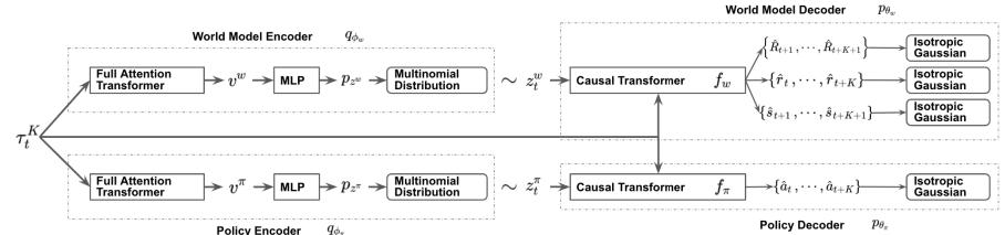
Similar to Decision Transformer, SPLT-Transformer is a sequence generation model using the Transformer architecture. But unlike the mentioned DT, it uses two separate information flows to model the Actor policy and the environment.
The method authors try to solve 2 main problems:
- Models should help create a variety of candidates for the Agent's behavior in any situation;
- Models should cover most of the different modes of potential transitions to a new environment state.
To achieve this goal, we train 2 separate VAEs based on Transformer for Actor policy and environment model. The method authors generate stochastic latent variables for both flows and use them over the entire planning horizon. This allows us to enumerate all possible candidate trajectories without exponentially increasing branching and provides an effective search for behavior options during testing.
The idea is that latent policy variables should correspond to different high-level intentions, similar to the skills of hierarchical algorithms. At the same time, the latent variables of the environmental model should correspond to various possible trends and the most likely change in its state.
The policy and environmental encoders use the same architecture using Transformers. They receive the same initial data in the form of a previous trajectory. But unlike the previously discussed algorithms, the trajectory includes only a set of Actor states and actions. At the output of the encoders, we obtain discrete latent variables with a limited number of values in each dimension.
The authors of the method propose to use the average value of the transformer outputs for all elements in order to combine the entire trajectory into one vector representation.
Next, each of these outputs is processed by a small multilayer perceptron that outputs independent categorical distributions of the latent representation.
The policy decoder receives the same original trajectory as input, supplemented by the corresponding latent representation. The goal of a policy decoder is to estimate probabilities and predict the next most likely next action in a trajectory. The authors of the method present a decoder using the Transformer model.
As mentioned above, we remove the reward from the sequence, but add a latent representation. However, the latent representation does not replace the reward as a sequence element at each step. The method authors introduce a latent representation transformed by a single embedding vector similar to the positional encoding used in some other works using the Transformer architecture.
The environment model decoder has an architecture similar to the policy decoder. At the output only, the environmental model decoder has "three heads" to predict the most likely subsequent state and its cost, as well as the transition reward.
As in DT, models are trained on data from the training set using supervised learning methods. Models are trained to compare trajectories with subsequent actions (Actor), transitions to new states and their costs (environmental model).
While testing and operation, the selection of the optimal action is carried out based on the assessment of candidate forecast trajectories at a given planning horizon. To compile one planned candidate trajectory, sequential generation of actions and states with rewards is carried out over the planning horizon. Then the optimal trajectory is selected and its first action is carried out. After the transition to a new state of the environment, the entire algorithm is repeated.
As you can see, the algorithm plans several candidate trajectories, but only one action of the optimal trajectory is performed. Although this approach may seem inefficient, it can minimize risks by planning several steps ahead. At the same time, it is possible to correct the trajectory in time as a result of re-evaluating each visited state.
The author's visualization of the method is presented below.
2. Implementation using MQL5
After considering the theoretical aspects of the SPLT-Transformer method, let's move on to implementing the proposed approaches using MQL5. I want to say right away that our implementation will be farther than ever from the author’s algorithm. The reason is my subjective perception. The entire experience of this series of articles demonstrates the complexity of creating an environmental model for financial markets. All our attempts yielded rather modest results. The accuracy of the forecasts is quite low at 1-2 steps. As the planning horizon grows, it tends to 0. Therefore, I decided not to build candidate trajectories, but to limit myself to only generating several candidate action options from the current state.
But this approach entails a gap between the action and its evaluation. As you can see in the visualization above, the Actor policy and the environmental model receive the same input data. But then the data flows in parallel streams. Therefore, when predicting the subsequent state and expected reward, the environmental model knows nothing about the action that the Agent will choose. Here we can only talk about a certain assumption with a certain degree of probability based on previous experience from the training sample. It should be noted that the training sample was created based on Actor policies different from those currently used one.
In the author’s version, this is leveled out by adding the Agent’s action and the forecast state to the trajectory at the next step. However, in our case, taking into account the experience of low quality planning for the subsequent state of the environment, we risk adding completely uncoordinated states and actions to the trajectory. This will lead to an even greater decrease in the quality of planning the next steps in the forecast trajectory. In my opinion, the efficiency of such planning and evaluation of such trajectories is very doubtful. Therefore, we will not waste resources on predicting candidate trajectories.
At the same time, we need a mechanism capable of comparing the Agent’s actions and the expected reward. On the one hand, we can use the Critic’s model, but this fundamentally breaks the algorithm and completely excludes the environmental model. Unless, of course, we use it as a Critic.
However, I decided to experiment with a different approach that is closer to the original algorithm. To begin with, I decided to use one encoder for both streams. The resulting latent state is added to the trajectory and fed to the input of 2 decoders. The actor, based on the initial data, generates a predictive action, and the environmental model returns the amount of the future discounted reward.
The idea is that, given the same input data, the models return consistent results. To do this, we exclude stochasticity in the Actor and environmental models. In doing so, we create stochasticity in the latent representation, which allows us to generate multiple candidate actions and associated predictive state estimates. Based on these estimates, we will rank candidate actions to select the optimal weighted step.
To optimize the number of operations performed, we should pay attention to one more point. By feeding the same trajectory to the Encoder input, we will repeat the results of all its internal layers with mathematical accuracy. Differences are formed only in the variational auto encoder layer when sampling from a given distribution. Therefore, to generate candidate actions, it is advisable for us to move the specified layer outside the Encoder. This will allow us to carry out only one Encoder pass at each iteration. After some thought, I moved the variational auto encoder layer into the environment model.
I went further along the path of optimizing the workflow. All three of our models use the same trajectory as input data. As you know, trajectory elements are not uniform. Before processing, they pass through an Embedding layer. This gave me the idea of embedding data in only one model, and then using the resulting data in the remaining two. Thus, I left the embedding layer only in the Encoder.
There is one more thing. The environment model and Actor use the concatenated vector of trajectory and latent representation as input. We have already determined that the variational auto encoder layer has been transferred to the environmental model for the formation of a stochastic latent representation. Here we will carry out the combination of vectors and pass the already obtained result to the Actor’s input.
Now let’s transfer the above ideas into the code. Let's create a description of our models. As always, it is formed in the CreateDescriptions method. In the parameters, the method receives pointers to three objects describing our models.
bool CreateDescriptions(CArrayObj *agent, CArrayObj *latent, CArrayObj *world)
  {
//---
   CLayerDescription *descr;
The description of the architecture should probably start with a model of an encoder whose input is supplied with unprocessed sequence data.
//---
   latent.Clear();
//--- Input layer
   if(!(descr = new CLayerDescription()))
      return false;
   descr.type = defNeuronBaseOCL;
   prev_count = descr.count = (BarDescr * NBarInPattern + AccountDescr + TimeDescription + NActions);
   descr.activation = None;
   descr.optimization = ADAM;
   if(!latent.Add(descr))
     {
      delete descr;
      return false;
     }
We pass the received data through a batch normalization layer to bring it into a comparable form.
//--- layer 1
   if(!(descr = new CLayerDescription()))
      return false;
   descr.type = defNeuronBatchNormOCL;
   descr.count = prev_count;
   descr.batch = 1000;
   descr.activation = None;
   descr.optimization = ADAM;
   if(!latent.Add(descr))
     {
      delete descr;
      return false;
     }
Pass the already normalized data through the embedding layer. Remember this layer. We will then take data from it into the environmental model.
//--- layer 2
   if(!(descr = new CLayerDescription()))
      return false;
   descr.type = defNeuronEmbeddingOCL;
   prev_count = descr.count = HistoryBars;
     {
      int temp[] = {BarDescr * NBarInPattern, AccountDescr, TimeDescription, NActions};
      ArrayCopy(descr.windows, temp);
     }
   int prev_wout = descr.window_out = EmbeddingSize;
   if(!latent.Add(descr))
     {
      delete descr;
      return false;
     }
Next, we carry out the resulting trajectory through the Transformer block. I used a sparse attention block with 8 Self-Attention heads and 4 layers per block.
//--- layer 3
   if(!(descr = new CLayerDescription()))
      return false;
   descr.type = defNeuronMLMHSparseAttentionOCL;
   prev_count = descr.count = prev_count * 4;
   descr.window = prev_wout;
   descr.step = 8;
   descr.window_out = 32;
   descr.layers = 4;
   descr.probability = Sparse;
   descr.optimization = ADAM;
   if(!latent.Add(descr))
     {
      delete descr;
      return false;
     }
After the attention block, we will slightly reduce the dimensionality of the convolutional layer and pass the data through a decision block from fully connected layers.
//--- layer 4
   if(!(descr = new CLayerDescription()))
      return false;
   descr.type = defNeuronConvOCL;
   descr.count = prev_count;
   descr.window = prev_wout;
   descr.step = prev_wout;
   descr.window_out = 4;
   descr.optimization = ADAM;
   descr.activation = LReLU;
   if(!latent.Add(descr))
     {
      delete descr;
      return false;
     }
//--- layer 5
   if(!(descr = new CLayerDescription()))
      return false;
   descr.type = defNeuronBaseOCL;
   descr.count = LatentCount;
   descr.optimization = ADAM;
   descr.activation = LReLU;
   if(!latent.Add(descr))
     {
      delete descr;
      return false;
     }
//--- layer 6
   if(!(descr = new CLayerDescription()))
      return false;
   descr.type = defNeuronBaseOCL;
   prev_count = descr.count = LatentCount;
   descr.activation = TANH;
   descr.optimization = ADAM;
   if(!latent.Add(descr))
     {
      delete descr;
      return false;
     }
//--- layer 7
   if(!(descr = new CLayerDescription()))
      return false;
   descr.type = defNeuronBaseOCL;
   descr.count = LatentCount;
   descr.activation = LReLU;
   descr.optimization = ADAM;
   if(!latent.Add(descr))
     {
      delete descr;
      return false;
     }
//--- layer 8
   if(!(descr = new CLayerDescription()))
      return false;
   descr.type = defNeuronBaseOCL;
   descr.count = 2 * EmbeddingSize;
   descr.activation = None;
   descr.optimization = ADAM;
   if(!latent.Add(descr))
     {
      delete descr;
      return false;
     }
At the output of the Encoder model, we use a fully connected neural layer without an activation function and with a size two times larger than the embedding size of one trajectory element. This is the means and variances for the latent representation distribution allowing us to sample the latent representation from a given distribution in the next step.
Next we move on to describe the environmental model. Its source data layer is equal to the results layer of the Encoder model and is followed by the variational auto encoder layer, which allows us to immediately sample the latent representation.
//--- World
   if(!world)
     {
      world = new CArrayObj();
      if(!world)
         return false;
     }
//---
   world.Clear();
//--- Input layer
   if(!(descr = new CLayerDescription()))
      return false;
   descr.type = defNeuronBaseOCL;
   prev_count = descr.count = 2 * EmbeddingSize;
   descr.activation = None;
   descr.optimization = ADAM;
   if(!world.Add(descr))
     {
      delete descr;
      return false;
     }
//--- layer 1
   if(!(descr = new CLayerDescription()))
      return false;
   descr.type = defNeuronVAEOCL;
   prev_count = descr.count = prev_count / 2;
   descr.activation = None;
   descr.optimization = ADAM;
   if(!world.Add(descr))
     {
      delete descr;
      return false;
     }
Next we have to add the trajectory embedding tensor. To do this, we will use a concatenation layer. At the output of this layer, we receive processed initial data for our environment model and Actor.
//--- layer 2
   if(!(descr = new CLayerDescription()))
      return false;
   descr.type = defNeuronConcatenate;
   descr.step = 4 * EmbeddingSize * HistoryBars;
   prev_count = descr.count = descr.step + prev_count;
   descr.activation = LReLU;
   descr.optimization = ADAM;
   if(!world.Add(descr))
     {
      delete descr;
      return false;
     }
Let's pass the data through the discharged Self-Attention block. As in the encoder, we use 8 heads and 4 layers.
//--- layer 3
   if(!(descr = new CLayerDescription()))
      return false;
   descr.type = defNeuronMLMHSparseAttentionOCL;
   prev_count = descr.count = prev_count / EmbeddingSize;
   descr.window = EmbeddingSize;
   descr.step = 8;
   descr.window_out = 32;
   descr.layers = 4;
   descr.probability = Sparse;
   descr.optimization = ADAM;
   if(!world.Add(descr))
     {
      delete descr;
      return false;
     }
Reduce the data dimensionality using a convolutional layer.
//--- layer 4
   if(!(descr = new CLayerDescription()))
      return false;
   descr.type = defNeuronConvOCL;
   descr.count = prev_count;
   descr.window = prev_wout;
   descr.step = prev_wout;
   descr.window_out = 4;
   descr.optimization = ADAM;
   descr.activation = LReLU;
   if(!world.Add(descr))
     {
      delete descr;
      return false;
     }
Process the received data with a fully connected perceptron of the decision-making block.
//--- layer 5
   if(!(descr = new CLayerDescription()))
      return false;
   descr.type = defNeuronBaseOCL;
   descr.count = LatentCount;
   descr.optimization = ADAM;
   descr.activation = LReLU;
   if(!world.Add(descr))
     {
      delete descr;
      return false;
     }
//--- layer 6
   if(!(descr = new CLayerDescription()))
      return false;
   descr.type = defNeuronBaseOCL;
   prev_count = descr.count = LatentCount;
   descr.activation = TANH;
   descr.optimization = ADAM;
   if(!world.Add(descr))
     {
      delete descr;
      return false;
     }
//--- layer 7
   if(!(descr = new CLayerDescription()))
      return false;
   descr.type = defNeuronBaseOCL;
   descr.count = LatentCount;
   descr.activation = LReLU;
   descr.optimization = ADAM;
   if(!world.Add(descr))
     {
      delete descr;
      return false;
     }
//--- layer 8
   if(!(descr = new CLayerDescription()))
      return false;
   descr.type = defNeuronBaseOCL;
   descr.count = NRewards;
   descr.activation = None;
   descr.optimization = ADAM;
   if(!world.Add(descr))
     {
      delete descr;
      return false;
     }
At the output of the model, we get a decomposed reward vector.
At the end of this block, we will look at the structure of our Actor model. As mentioned above, the model receives its initial data from the hidden state of the environmental model. Accordingly, the source data layer should be of sufficient size.
//---
   if(!agent)
     {
      agent = new CArrayObj();
      if(!agent)
         return false;
     }
//--- Agent
   agent.Clear();
//--- Input layer
   if(!(descr = new CLayerDescription()))
      return false;
   descr.type = defNeuronBaseOCL;
   int prev_count = descr.count = EmbeddingSize * (4 * HistoryBars + 1);
   descr.activation = None;
   descr.optimization = ADAM;
   if(!agent.Add(descr))
     {
      delete descr;
      return false;
     }
The obtained data is the result of the model and does not require additional processing. Therefore, we immediately use the sparse attention block. The block parameters are similar to those used in the models discussed above. Thus, all three models use the same transformer architecture.
//--- layer 1
   if(!(descr = new CLayerDescription()))
      return false;
   descr.type = defNeuronMLMHSparseAttentionOCL;
   prev_count = descr.count = prev_count / EmbeddingSize;
   descr.window = EmbeddingSize;
   descr.step = 8;
   descr.window_out = 32;
   descr.layers = 4;
   descr.probability = Sparse;
   descr.optimization = ADAM;
   if(!agent.Add(descr))
     {
      delete descr;
      return false;
     }
Similar to the environmental model, we reduce the dimensionality and process the data in a fully connected decision perceptron.
//--- layer 2
   if(!(descr = new CLayerDescription()))
      return false;
   descr.type = defNeuronConvOCL;
   descr.count = prev_count;
   descr.window = EmbeddingSize;
   descr.step = EmbeddingSize;
   descr.window_out = 4;
   descr.optimization = ADAM;
   descr.activation = LReLU;
   if(!agent.Add(descr))
     {
      delete descr;
      return false;
     }
//--- layer 3
   if(!(descr = new CLayerDescription()))
      return false;
   descr.type = defNeuronBaseOCL;
   descr.count = LatentCount;
   descr.optimization = ADAM;
   descr.activation = LReLU;
   if(!agent.Add(descr))
     {
      delete descr;
      return false;
     }
//--- layer 4
   if(!(descr = new CLayerDescription()))
      return false;
   descr.type = defNeuronBaseOCL;
   prev_count = descr.count = LatentCount;
   descr.activation = TANH;
   descr.optimization = ADAM;
   if(!agent.Add(descr))
     {
      delete descr;
      return false;
     }
//--- layer 5
   if(!(descr = new CLayerDescription()))
      return false;
   descr.type = defNeuronBaseOCL;
   descr.count = LatentCount;
   descr.activation = LReLU;
   descr.optimization = ADAM;
   if(!agent.Add(descr))
     {
      delete descr;
      return false;
     }
//--- layer 6
   if(!(descr = new CLayerDescription()))
      return false;
   descr.type = defNeuronBaseOCL;
   descr.count = NActions;
   descr.activation = SIGMOID;
   descr.optimization = ADAM;
   if(!agent.Add(descr))
     {
      delete descr;
      return false;
     }
//---
   return true;
  }
At the output of the model, a vector of Agent actions is formed.
We also need to pay attention that to implement this method, we will need to add an additional entity to the experience playback buffer in the form of a distribution of the latent representation, which is formed at the output of the Encoder. To do this, we will create an additional array in the structure of describing the environment state.
struct SState
  {
.......
.......
   float             latent[2 * EmbeddingSize];
.......
.......
  }
The size of the new array is equal to two embeddings, since it includes the average values and variances of the distribution.
In addition to declaring the array, we need to add its maintenance to all structure methods:
- Initialization with initial values
SState::SState(void)
  {
.......
.......
   ArrayInitialize(latent, 0);
  }
- Cleaning the structure
   void              Clear(void)
     {
.......
.......
      ArrayInitialize(latent, 0);
     }
- Copying the structure
   void              operator=(const SState &obj)
     {
.......
.......
      ArrayCopy(latent, obj.latent);
     }
- Saving the structure
bool SState::Save(int file_handle)
  {
.......
.......
//---
   total = ArraySize(latent);
   if(FileWriteInteger(file_handle, total) < sizeof(int))
      return false;
   for(int i = 0; i < total; i++)
      if(FileWriteFloat(file_handle, latent[i]) < sizeof(float))
         return false;
//---
   return true;
  }
- Uploading the structure from the file
bool SState::Load(int file_handle)
  {
.......
.......
//---
   total = FileReadInteger(file_handle);
   if(total != ArraySize(latent))
      return false;
//---
   for(int i = 0; i < total; i++)
     {
      if(FileIsEnding(file_handle))
         return false;
      latent[i] = FileReadFloat(file_handle);
     }
//---
   return true;
  }
We got acquainted with the architecture of trained models and updated the data structure. The next step is to collect data for their training. This functionality is performed in the "...\SPLT\Research.mq5" EA. The SPLT-Transformer method provides generation of candidate trajectories (or candidate actions in our implementation). The number of such candidates is one of the hyperparameters of the model, which we include in the EA external parameters.
input int Agents = 5;
As you might remember, earlier we used the Agents external parameter as an auxiliary parameter to indicate the number of parallel environmental research agents in the optimization mode of the strategy tester. Now we will rename the EA service parameter.
input int OptimizationAgents = 1;
Further on, we will not dwell in detail on all EA methods for collecting a training sample. Their algorithm has already been described many times in this series. The full code of all programs used in the article is available in the attachment. Let's consider only the OnTick method of direct interaction with the environment, which contains the key features of the implemented algorithm.
At the beginning of the method, we, as usual, check the occurrence of the new bar opening event and, if necessary, update the historical data of price movement and indicators of the analyzed indicators.
//+------------------------------------------------------------------+
//| Expert tick function                                             |
//+------------------------------------------------------------------+
void OnTick()
  {
//---
   if(!IsNewBar())
      return;
//---
   int bars = CopyRates(Symb.Name(), TimeFrame, iTime(Symb.Name(), TimeFrame, 1), NBarInPattern, Rates);
   if(!ArraySetAsSeries(Rates, true))
      return;
//---
   RSI.Refresh();
   CCI.Refresh();
   ATR.Refresh();
   MACD.Refresh();
   Symb.Refresh();
   Symb.RefreshRates();
After that, we create a buffer of source data for the models. First, we enter historical data on price movement and the values of the analyzed indicators.
//+------------------------------------------------------------------+
//| Expert tick function                                             |
//+------------------------------------------------------------------+
void OnTick()
  {
//---
   if(!IsNewBar())
      return;
//---
   int bars = CopyRates(Symb.Name(), TimeFrame, iTime(Symb.Name(), TimeFrame, 1), NBarInPattern, Rates);
   if(!ArraySetAsSeries(Rates, true))
      return;
//---
   RSI.Refresh();
   CCI.Refresh();
   ATR.Refresh();
   MACD.Refresh();
   Symb.Refresh();
   Symb.RefreshRates();
//--- History data
   float atr = 0;
   for(int b = 0; b < (int)NBarInPattern; b++)
     {
      float open = (float)Rates[b].open;
      float rsi = (float)RSI.Main(b);
      float cci = (float)CCI.Main(b);
      atr = (float)ATR.Main(b);
      float macd = (float)MACD.Main(b);
      float sign = (float)MACD.Signal(b);
      if(rsi == EMPTY_VALUE || cci == EMPTY_VALUE || atr == EMPTY_VALUE || macd == EMPTY_VALUE || sign == EMPTY_VALUE)
         continue;
      //---
      int shift = b * BarDescr;
      sState.state[shift] = (float)(Rates[b].close - open);
      sState.state[shift + 1] = (float)(Rates[b].high - open);
      sState.state[shift + 2] = (float)(Rates[b].low - open);
      sState.state[shift + 3] = (float)(Rates[b].tick_volume / 1000.0f);
      sState.state[shift + 4] = rsi;
      sState.state[shift + 5] = cci;
      sState.state[shift + 6] = atr;
      sState.state[shift + 7] = macd;
      sState.state[shift + 8] = sign;
     }
   bState.AssignArray(sState.state);
Then we will add the current account status and information about open positions.
//--- Account description
   sState.account[0] = (float)AccountInfoDouble(ACCOUNT_BALANCE);
   sState.account[1] = (float)AccountInfoDouble(ACCOUNT_EQUITY);
//---
   double buy_value = 0, sell_value = 0, buy_profit = 0, sell_profit = 0;
   double position_discount = 0;
   double multiplyer = 1.0 / (60.0 * 60.0 * 10.0);
   int total = PositionsTotal();
   datetime current = TimeCurrent();
   for(int i = 0; i < total; i++)
     {
      if(PositionGetSymbol(i) != Symb.Name())
         continue;
      double profit = PositionGetDouble(POSITION_PROFIT);
      switch((int)PositionGetInteger(POSITION_TYPE))
        {
         case POSITION_TYPE_BUY:
            buy_value += PositionGetDouble(POSITION_VOLUME);
            buy_profit += profit;
            break;
         case POSITION_TYPE_SELL:
            sell_value += PositionGetDouble(POSITION_VOLUME);
            sell_profit += profit;
            break;
        }
      position_discount += profit - (current - PositionGetInteger(POSITION_TIME)) * multiplyer * MathAbs(profit);
     }
   sState.account[2] = (float)buy_value;
   sState.account[3] = (float)sell_value;
   sState.account[4] = (float)buy_profit;
   sState.account[5] = (float)sell_profit;
   sState.account[6] = (float)position_discount;
   sState.account[7] = (float)Rates[0].time;
//---
   bState.Add((float)((sState.account[0] - PrevBalance) / PrevBalance));
   bState.Add((float)(sState.account[1] / PrevBalance));
   bState.Add((float)((sState.account[1] - PrevEquity) / PrevEquity));
   bState.Add(sState.account[2]);
   bState.Add(sState.account[3]);
   bState.Add((float)(sState.account[4] / PrevBalance));
   bState.Add((float)(sState.account[5] / PrevBalance));
   bState.Add((float)(sState.account[6] / PrevBalance));
Next, we perform temporal identification of the data by adding a timestamp to our data buffer.
//--- Time label
   double x = (double)Rates[0].time / (double)(D'2024.01.01' - D'2023.01.01');
   bState.Add((float)MathSin(2.0 * M_PI * x));
   x = (double)Rates[0].time / (double)PeriodSeconds(PERIOD_MN1);
   bState.Add((float)MathCos(2.0 * M_PI * x));
   x = (double)Rates[0].time / (double)PeriodSeconds(PERIOD_W1);
   bState.Add((float)MathSin(2.0 * M_PI * x));
   x = (double)Rates[0].time / (double)PeriodSeconds(PERIOD_D1);
   bState.Add((float)MathSin(2.0 * M_PI * x));
Indicate the last actions of the Agent that brought us into this state of the environment.
//--- Prev action
   bState.AddArray(AgentResult);
The collected data about the current step is enough to generate a latent representation and we call the Encoder's forward pass method. At the same time, we make sure to monitor performed operations. Inform the user if necessary.
//--- Latent representation
   ResetLastError();
   if(!Latent.feedForward(GetPointer(bState), 1, false))
     {
      PrintFormat("Error of Latent model feed forward: %d",GetLastError());
      return;
     }
After successfully creating the latent representation, we move on to our decoders.
Let me remind you that at this stage we have to generate candidate actions. We will form them in a loop. Its number of iterations will be equal to the number of required candidates and will be indicated in the EA external parameters.
To save information about the generated candidate actions, we will create the actions and values matrices. In the first one, we will record action vectors. The second one is to contain the expected rewards as a result of applying the policy.
As mentioned above, in the Encoder model, we only generate data on the distribution of the latent representation. Sampling of the latent representation vector is carried out in the environmental model. Therefore, in the body of the loop, we first perform a forward pass through the environment model. Then we call the Agent's forward pass method, which uses the hidden states of the environmental model as input.
The results of direct passes of the models are saved into previously prepared matrices.
   matrix<float> actions = matrix<float>::Zeros(Agents, NActions);
   matrix<float> values = matrix<float>::Zeros(Agents, NRewards);
   for(ulong i = 0; i < (ulong)Agents; i++)
     {
      if(!World.feedForward(GetPointer(Latent), -1, GetPointer(Latent), LatentLayer) ||
         !Agent.feedForward(GetPointer(World), 2,(CBufferFloat *)NULL))
         return;
      vector<float> result;
      Agent.getResults(result);
      actions.Row(result, i);
      World.getResults(result);
      values.Row(result, i);
     }
The use of stochastic policies is based on the assumption of an equal probability of occurrence of one of the events within the learned distribution. Therefore, each sampled candidate action has an equal probability of receiving the expected reward in the environment. Our goal is to obtain maximum profitability. This means that under conditions of equal probability, we choose the action with the maximum expected return.
As you understand, our matrices are row-correlated. We are looking for the row with the maximum expected reward in the values matrix and select an action from the corresponding row of the actions matrix.
   vector<float> temp = values.Sum(1);
   temp = actions.Row(temp.ArgMax());
The selected action takes place in the environment.
//---
   PrevBalance = sState.account[0];
   PrevEquity = sState.account[1];
//---
   double min_lot = Symb.LotsMin();
   double step_lot = Symb.LotsStep();
   double stops = MathMax(Symb.StopsLevel(), 1) * Symb.Point();
   if(temp[0] >= temp[3])
     {
      temp[0] -= temp[3];
      temp[3] = 0;
     }
   else
     {
      temp[3] -= temp[0];
      temp[0] = 0;
     }
   float delta = MathAbs(AgentResult - temp).Sum();
   AgentResult = temp;
//--- buy control
   if(temp[0] < min_lot || (temp[1] * MaxTP * Symb.Point()) <= stops || (temp[2] * MaxSL * Symb.Point()) <= stops)
     {
      if(buy_value > 0)
         CloseByDirection(POSITION_TYPE_BUY);
     }
   else
     {
      double buy_lot = min_lot + MathRound((double)(temp[0] - min_lot) / step_lot) * step_lot;
      double buy_tp = Symb.NormalizePrice(Symb.Ask() + temp[1] * MaxTP * Symb.Point());
      double buy_sl = Symb.NormalizePrice(Symb.Ask() - temp[2] * MaxSL * Symb.Point());
      if(buy_value > 0)
         TrailPosition(POSITION_TYPE_BUY, buy_sl, buy_tp);
      if(buy_value != buy_lot)
        {
         if(buy_value > buy_lot)
            ClosePartial(POSITION_TYPE_BUY, buy_value - buy_lot);
         else
            Trade.Buy(buy_lot - buy_value, Symb.Name(), Symb.Ask(), buy_sl, buy_tp);
        }
     }
//--- sell control
   if(temp[3] < min_lot || (temp[4] * MaxTP * Symb.Point()) <= stops || (temp[5] * MaxSL * Symb.Point()) <= stops)
     {
      if(sell_value > 0)
         CloseByDirection(POSITION_TYPE_SELL);
     }
   else
     {
      double sell_lot = min_lot + MathRound((double)(temp[3] - min_lot) / step_lot) * step_lot;;
      double sell_tp = Symb.NormalizePrice(Symb.Bid() - temp[4] * MaxTP * Symb.Point());
      double sell_sl = Symb.NormalizePrice(Symb.Bid() + temp[5] * MaxSL * Symb.Point());
      if(sell_value > 0)
         TrailPosition(POSITION_TYPE_SELL, sell_sl, sell_tp);
      if(sell_value != sell_lot)
        {
         if(sell_value > sell_lot)
            ClosePartial(POSITION_TYPE_SELL, sell_value - sell_lot);
         else
            Trade.Sell(sell_lot - sell_value, Symb.Name(), Symb.Bid(), sell_sl, sell_tp);
        }
     }
The results of interaction with the environment are collected into a previously prepared structure and stored in the experience playback buffer.
//---
   int shift = BarDescr * (NBarInPattern - 1);
   sState.rewards[0] = bState[shift];
   sState.rewards[1] = bState[shift + 1] - 1.0f;
   if((buy_value + sell_value) == 0)
      sState.rewards[2] -= (float)(atr / PrevBalance);
   else
      sState.rewards[2] = 0;
   for(ulong i = 0; i < NActions; i++)
      sState.action[i] = AgentResult[i];
   Latent.getResults(sState.latent);
   if(!Base.Add(sState))
      ExpertRemove();
  }
This concludes our introduction the EA for interacting with the environment and collecting training sample data. You can find its full code in the attachment. There you will also find the complete code of all programs used in the article. We are moving on to offline model training EA "...\SPLT\Study.mq5".
In the EA initialization method, we first upload the training set. Make sure to control the operations. For offline model training, this is the only source of data and its absence makes the rest of the process impossible.
//+------------------------------------------------------------------+
//| Expert initialization function                                   |
//+------------------------------------------------------------------+
int OnInit()
  {
//---
   ResetLastError();
   if(!LoadTotalBase())
     {
      PrintFormat("Error of load study data: %d", GetLastError());
      return INIT_FAILED;
     }
Next, we try to load the pre-trained models and create new ones if necessary.
//--- load models
   float temp;
   if(!Agent.Load(FileName + "Act.nnw", temp, temp, temp, dtStudied, true) ||
      !World.Load(FileName + "Wld.nnw", temp, temp, temp, dtStudied, true) ||
      !Latent.Load(FileName + "Lat.nnw", temp, temp, temp, dtStudied, true))
     {
      CArrayObj *agent = new CArrayObj();
      CArrayObj *latent = new CArrayObj();
      CArrayObj *world = new CArrayObj();
      if(!CreateDescriptions(agent, latent, world))
        {
         delete agent;
         delete latent;
         delete world;
         return INIT_FAILED;
        }
      if(!Agent.Create(agent) ||
         !World.Create(world) ||
         !Latent.Create(latent))
        {
         delete agent;
         delete latent;
         delete world;
         return INIT_FAILED;
        }
      delete agent;
      delete latent;
      delete world;
      //---
     }
As you may have noticed, the algorithm of the EA for collecting a training sample often uses data transfer between trained models. During the training process, the volume of transmitted data increases, because the data flow is carried out in two directions: forward and reverse passes. In order to eliminate unnecessary data copying operations between the OpenCL context and main memory, we will transfer all models to a single OpenCL context.
   COpenCL *opcl = Agent.GetOpenCL();
   Latent.SetOpenCL(opcl);
   World.SetOpenCL(opcl);
Next, we check the consistency of the architecture of the trained models.
   Agent.getResults(Result);
   if(Result.Total() != NActions)
     {
      PrintFormat("The scope of the Agent does not match the actions count (%d <> %d)", 6, Result.Total());
      return INIT_FAILED;
     }
//---
   Latent.GetLayerOutput(0, Result);
   if(Result.Total() != (BarDescr * NBarInPattern + AccountDescr + TimeDescription + NActions))
     {
      PrintFormat("Input size of Latent model doesn't match state description (%d <> %d)",
                   Result.Total(), (BarDescr * NBarInPattern + AccountDescr + TimeDescription + NActions));
      return INIT_FAILED;
     }
   Latent.Clear();
After successful completion of all controls, we generate an event for the start of model training and complete the operation of the EA initialization method.
//---
   if(!EventChartCustom(ChartID(), 1, 0, 0, "Init"))
     {
      PrintFormat("Error of create study event: %d", GetLastError());
      return INIT_FAILED;
     }
//---
   return(INIT_SUCCEEDED);
  }
The actual process of training models is arranged in the Train method. In the body of the method, we determine the number of trajectories in the experience playback buffer and record the start time of training in a local variable. It will serve as a guide for us to periodically inform the user about the model training progress.
//+------------------------------------------------------------------+
//| Train function                                                   |
//+------------------------------------------------------------------+
void Train(void)
  {
   int total_tr = ArraySize(Buffer);
   uint ticks = GetTickCount();
Let me remind you that our models use the GPT architecture, which is sensitive to the sequence of the source data. As before in similar cases, we will use a nested loop system to train models. In the external loop, we sample the trajectory from the experience replay buffer and the initial state of the environment.
   bool StopFlag = false;
   for(int iter = 0; (iter < Iterations && !IsStopped() && !StopFlag); iter ++)
     {
      int tr = (int)((MathRand() / 32767.0) * (total_tr - 1));
      int i = (int)((MathRand() * MathRand() / MathPow(32767, 2)) *
                     MathMax(Buffer[tr].Total - 2 * HistoryBars,MathMin(Buffer[tr].Total,20)));
      if(i < 0)
        {
         iter--;
         continue;
        }
Then we initialize the model buffers and create a nested loop, in which we sequentially feed a separate fragment of historical data as the model input.
      Actions = vector<float>::Zeros(NActions);
      Latent.Clear();
      for(int state = i; state < MathMin(Buffer[tr].Total - 2,i + HistoryBars * 3); state++)
        {
In the body of a nested loop, operations can be somewhat reminiscent of collecting training data. We also fill the source data buffer. Only now we do not request data from the environment, but extract it from the experience playback buffer. At the same time, we strictly observe the sequence of data recording. First, we enter information about price movement and indicators of the analyzed indicators into the source data buffer.
         //--- History data
         State.AssignArray(Buffer[tr].States[state].state);
Then there is data about the account status and open positions.
         //--- Account description
         float PrevBalance = (state == 0 ? Buffer[tr].States[state].account[0] : Buffer[tr].States[state - 1].account[0]);
         float PrevEquity = (state == 0 ? Buffer[tr].States[state].account[1] : Buffer[tr].States[state - 1].account[1]);
         State.Add((Buffer[tr].States[state].account[0] - PrevBalance) / PrevBalance);
         State.Add(Buffer[tr].States[state].account[1] / PrevBalance);
         State.Add((Buffer[tr].States[state].account[1] - PrevEquity) / PrevEquity);
         State.Add(Buffer[tr].States[state].account[2]);
         State.Add(Buffer[tr].States[state].account[3]);
         State.Add(Buffer[tr].States[state].account[4] / PrevBalance);
         State.Add(Buffer[tr].States[state].account[5] / PrevBalance);
         State.Add(Buffer[tr].States[state].account[6] / PrevBalance);
The data identified by a timestamp.
         //--- Time label
         double x = (double)Buffer[tr].States[state].account[7] / (double)(D'2024.01.01' - D'2023.01.01');
         State.Add((float)MathSin(2.0 * M_PI * x));
         x = (double)Buffer[tr].States[state].account[7] / (double)PeriodSeconds(PERIOD_MN1);
         State.Add((float)MathCos(2.0 * M_PI * x));
         x = (double)Buffer[tr].States[state].account[7] / (double)PeriodSeconds(PERIOD_W1);
         State.Add((float)MathSin(2.0 * M_PI * x));
         x = (double)Buffer[tr].States[state].account[7] / (double)PeriodSeconds(PERIOD_D1);
         State.Add((float)MathSin(2.0 * M_PI * x));
Make sure to indicate the actions of the Agent that led us to this state.
         //--- Prev action
         State.AddArray(Actions);
Once again I want to emphasize strict adherence to consistency. The buffer data is not named. The model evaluates the data according to its position in the buffer. A change in sequence is perceived by the model as a completely different state. The result of the decision will be completely different and unpredictable. Therefore, in order not to confuse the model and always obtain adequate solutions, we need to strictly observe the sequence of data at all stages of training and operating the model.
After collecting the raw data buffer, we first perform a forward pass of the Encoder and the environment model.
         //--- Latent and Wordl
         if(!Latent.feedForward(GetPointer(State)) ||
            !World.feedForward(GetPointer(Latent), -1, GetPointer(Latent), LatentLayer))
           {
            PrintFormat("%s -> %d", __FUNCTION__, __LINE__);
            StopFlag = true;
            break;
           }
Note that we do not generate candidate actions during training. Moreover, training of the environmental model and the Actor's policy is carried out separately. This is due to the specifics of model training.
The environmental model is trained to estimate the Agent's policy based on the previous trajectory and predict the receipt of reward in the future, taking into account the current state of the environment and the policy used. At the same time, we adjust the distribution of the latent representation. To do this, after a successful forward pass, we perform a backward pass of the environmental model and encoder, aimed at minimizing the prediction error of the environmental model and the actual reward from the experience playback buffer.
         Actions.Assign(Buffer[tr].States[state].rewards);
         vector<float> result;
         World.getResults(result);
         Result.AssignArray(CAGrad(Actions - result) + result);
         if(!World.backProp(Result,GetPointer(Latent),LatentLayer) ||
            !Latent.backPropGradient((CBufferFloat *)NULL,(CBufferFloat *)NULL,LatentLayer) ||
            !Latent.backPropGradient((CBufferFloat *)NULL,(CBufferFloat *)NULL))
           {
            PrintFormat("%s -> %d", __FUNCTION__, __LINE__);
            StopFlag = true;
            break;
           }
Please note that after the environment model backpass, we first perform a partial Encoder backpass to optimize the Embedding parameters to suit the environment model's requirements. Then we perform a full reverse pass of the Encoder, during which the distribution of the latent representation is optimized.
We optimize the Actor Policy to match the latent state and the executed action. Therefore, we extract the latent representation distribution from the experience replay buffer and feed it into the input of the environmental model to resample the latent representation. Next, we carry out a direct pass of the environment models and the Actor.
         //--- Policy Feed Forward
         Result.AssignArray(Buffer[tr].States[state+1].latent);
         Latent.GetLayerOutput(LatentLayer,Result2);
         if(Result2.GetIndex()>=0)
            Result2.BufferWrite();
         if(!World.feedForward(Result, 1, false, Result2) ||
            !Agent.feedForward(GetPointer(World),2,(CBufferFloat *)NULL))
           {
            PrintFormat("%s -> %d", __FUNCTION__, __LINE__);
            StopFlag = true;
            break;
           }
Then we perform a reverse pass of the Actor to minimize the error between the predicted action and the one actually performed from the experience playback buffer.
         //--- Policy study
         Actions.Assign(Buffer[tr].States[state].action);
         Agent.getResults(result);
         Result.AssignArray(CAGrad(Actions - result) + result);
         if(!Agent.backProp(Result,NULL,NULL))
           {
            PrintFormat("%s -> %d", __FUNCTION__, __LINE__);
            StopFlag = true;
            break;
           }
In this way, we train the Actor's policy and make it more predictable. At the same time, we train an environmental model to evaluate previous trajectories to understand profitability. We train the Encoder to distill incoming trajectories to extract basic information about environmental trends and the current policies of the Actor.
All this together allows us to create quite interesting Actor policies, taking into account the stochasticity of the environment and the probabilities of making a profit.
Once the model update operations are successfully completed, we inform the user about the training progress and move on to the next iteration of our nested loop system.
         if(GetTickCount() - ticks > 500)
           {
            string str = StringFormat("%-15s %5.2f%% -> Error %15.8f\n", "Agent",
                                      iter * 100.0 / (double)(Iterations), Agent.getRecentAverageError());
            str += StringFormat("%-15s %5.2f%% -> Error %15.8f\n", "World",
                                      iter * 100.0 / (double)(Iterations), World.getRecentAverageError());
            Comment(str);
            ticks = GetTickCount();
           }
        }
     }
Once all iterations of the loop system are complete, we clear the comment field. Model training results are displayed in a journal. Initiate the EA termination.
   Comment("");
//---
   PrintFormat("%s -> %d -> %-15s %10.7f", __FUNCTION__, __LINE__, "Agent", Agent.getRecentAverageError());
   PrintFormat("%s -> %d -> %-15s %10.7f", __FUNCTION__, __LINE__, "World", World.getRecentAverageError());
   ExpertRemove();
//---
  }
This concludes our consideration of the Model Training EA for our interpretation of the SPLT-Transformer method. The full code of the EA and all programs used in the article is available in the attachment. There you can also find the code for the "...\SPLT\Test.mq5" model testing EA. We will not dwell on its methods in this article. The EA structure repeats the previously discussed similar EAs from previous articles. The implementation features of the presented algorithm in the OnTick function completely repeat the implementation of a similar method in the data collection EA for the training sample. I suggest you familiarize yourself with this EA in the attached files.
We are moving on to the next stage - testing models on historical data in the MetaTrader 5 strategy tester.
3. Testing
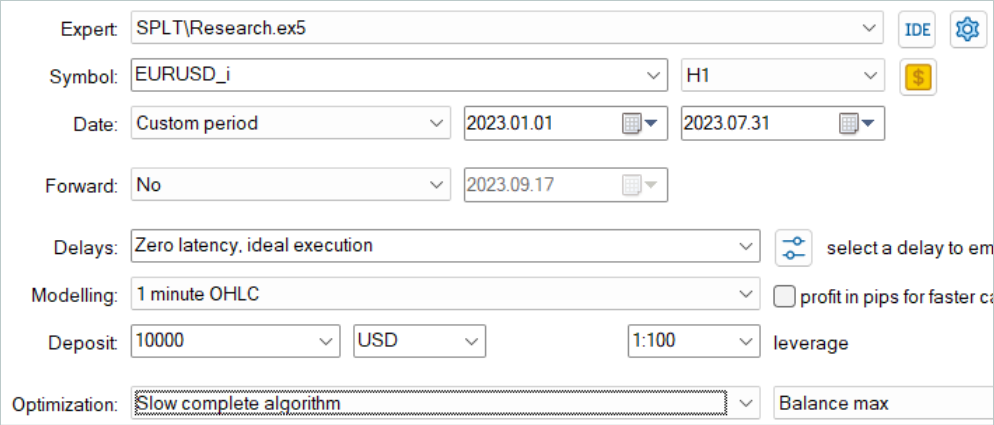
The models were trained on historical data for the first 7 months on EURUSD H1. The default parameters of all indicators are used without any additional optimization.
First, we launch the training sample collection EA in the slow optimization mode of the strategy tester. This allows us to collect data in parallel by several test agents. Thus, we increase the number of trajectories in the experience playback buffer while minimizing the time spent on data collection.
The considered algorithm assumes that models are trained only offline. Therefore, to test its performance, I suggest maximizing the experience playback buffer and filling it with a variety of trajectories. But it is worth noting that generating candidate actions is a rather expensive process. As the number of candidates increases, so do the costs of data collection.
After collecting the data, I trained the models without additionally collecting trajectories, as was done previously. Training a model, as always, is a long process. Since I did not plan additional collection of trajectories, I increased the number of trajectories and left my computer for long-term training.
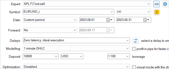
Next, the trained model was tested on historical data for August 2023, which was not included in the training set.
Based on the test results, the model showed a small profit and fairly accurate trading. Let me remind you that the SPLT-Transformer method was developed for autonomous driving and provides for maximum risk reduction.
On the test graph, we see a tendency for the balance to grow almost throughout the entire month. A series of unprofitable trades is observed only in the last week of the month. However, the previously accumulated profits were enough to cover losses. Overall, a small profit was recorded at the end of the month.


During the entire test period, the model opened only 16 positions with a minimum volume. The share of profitable trades is only 37.5%. However, the average winning trade is almost 70% greater than the average loss. As a result, the profit factor is 1.02 according to the test results.
Conclusion
In this paper, we presented SPLT-Transformer, an innovative method that was developed to solve problems in offline reinforcement learning associated with optimistic Agent behavior. The construction of reliable and efficient Agent policies is achieved using two separate models representing the policy and the world model.
The core components of SPLT-Transformer, including the candidate trajectory generation algorithm, allow us to simulate a variety of scenarios and make decisions taking into account a variety of possible future outcomes. This makes the presented method highly adaptive and safe in various stochastic environments. The method authors provided experimental results in the field of autonomous driving, confirming the superior performance of SPLT-Transformer in comparison with existing methods.
In the practical part of the article, we created our own, slightly simplified interpretation of the method discussed. We trained and tested the resulting models. The test results demonstrated that the model is capable of demonstrating both cautious and optimistic behavior depending on the situation. This makes it an ideal choice for mission-critical systems.
Overall, the method deserves further development. More thorough training of models, in my opinion, can give better results.
I remind you once again that all the programs presented in this series of articles were created only to demonstrate and test the algorithms in question. They are not suitable for trading on real accounts. Before using a particular model in real trading, it is recommended that it be thoroughly trained and tested.
Links
- Addressing Optimism Bias in Sequence Modeling for Reinforcement Learning
- Neural networks made easy (Part 58): Decision Transformer (DT)
- Neural networks are easy (Part 59): Dichotomy of Control (DoC)
- Neural networks made easy (Part 60): Online Decision Transformer (ODT)
Programs used in the article
| # | Name | Type | Description |
|---|---|---|---|
| 1 | Research.mq5 | Expert Advisor | Example collection EA |
| 2 | Study.mq5 | Expert Advisor | Agent training EA |
| 3 | Test.mq5 | Expert Advisor | Model testing EA |
| 4 | Trajectory.mqh | Class library | System state description structure |
| 5 | NeuroNet.mqh | Class library | A library of classes for creating a neural network |
| 6 | NeuroNet.cl | Code Base | OpenCL program code library |
Translated from Russian by MetaQuotes Ltd.
Original article: https://www.mql5.com/ru/articles/13639
Warning: All rights to these materials are reserved by MetaQuotes Ltd. Copying or reprinting of these materials in whole or in part is prohibited.
This article was written by a user of the site and reflects their personal views. MetaQuotes Ltd is not responsible for the accuracy of the information presented, nor for any consequences resulting from the use of the solutions, strategies or recommendations described.

 Deep Learning GRU model with Python to ONNX with EA, and GRU vs LSTM models
- Free trading apps
- Over 8,000 signals for copying
- Economic news for exploring financial markets
You agree to website policy and terms of use
Neural Networks - It's Simple (Part 61)
Part 61, can you see the result in monetary terms?
Neural networks are easy (Part 61)
61 parts, can you see the result in monetary terms?
I must say a big thank you to the author, who takes a purely theoretical article and explains in popular language how it can:
Take a look at the original article and see for yourself what kind of work Dmitry has done - https://arxiv.org/abs/2207.10295.