
Neural networks made easy (Part 39): Go-Explore, a different approach to exploration

Introduction
We continue the theme of environmental exploration in reinforcement learning. In previous articles within this series, we have already looked at algorithms for exploring the environment through curiosity and disagreement in an ensemble of models. Both approaches exploited intrinsic rewards to motivate the agent to perform different actions in similar situations while exploring new areas. But the problem is that the intrinsic reward decreases as the environment gets better explored. In complex cases of rare rewards, or when the agent may receive penalties on the way to the reward, this approach may not be very effective. In this article, I propose to get acquainted with a slightly different approach to studying the environment – the Go-Explore algorithm.
1. Go-Explore algorithm
Go-Explore is a reinforcement learning algorithm designed to find optimal solutions to complex problems that have a large action and state space. The algorithm was developed by Adrien Ecoffet and was described in the article Go-Explore: a New Approach for Hard-Exploration Problems.
He uses evolutionary algorithms and machine learning techniques to efficiently find optimal solutions to complex and intractable problems.
The algorithm begins by exploring a large number of random paths, called "base explorations". Then, using an evolutionary algorithm, it stores the best solutions found and combines them to create new paths. These new paths are then compared to the previous best solutions, and if they are better, they are saved. This process is repeated until the optimal solution is found.
Go-Explore also uses a technique called "recorder" to save the best solutions found and reuse them to create new paths. This allows the algorithm to find better solutions than if it simply continued to explore random paths.
One of the main advantages of Go-Explore is its ability to find optimal solutions in complex and intractable problems where other reinforcement learning algorithms might fail. It is also capable of learning efficiently under sparse rewards, which can be a challenge for other algorithms.
Overall, Go-Explore is a powerful tool for solving reinforcement learning problems and can be effectively applied in various fields, including robotics, computer games, and artificial intelligence in general.
The main idea of Go-Explore is to remember and return to promising states. This is fundamental for effective operation when the number of rewards is limited. This idea is so flexible and broad that it can be implemented in a variety of ways.
Unlike most reinforcement learning algorithms, Go-Explore does not focus on directly solving the target problem, but rather on finding relevant states and actions in the state space that can lead to achieving the target state. To achieve this, the algorithm has two main phases: search and reuse.
The first phase is to go through all the states in the state space and record each state visited in a state "map". After this, the algorithm begins to study each visited state in more detail and to collect information about actions that can lead to other interesting states.
The second phase is to reuse previously learned states and actions to find new solutions. The algorithm stores the most successful trajectories and uses them to generate new states that can lead to even more successful solutions.
The Go-Explore algorithm works as follows:
- Collecting an archive of examples: The agent starts the game, records each achievement, and saves it in the archive. Instead of storing the states themselves, the archive contains descriptions of the actions that led to the achievement of a particular state.
- Iterative exploration: At each iteration, the agent selects a random state from the archive and replays the game from this state. It saves any new states it manages to achieve and adds them to the archive along with a description of the actions that led to those states.
- Example-based learning: After iterative exploration, the algorithm learns from the examples it has collected using some kind of reinforcement learning algorithm.
- Repeat: The algorithm repeats iterative exploration and example-based learning until it reaches the desired level of performance.
The goal of the Go-Explore algorithm is to minimize the number of game replays required to achieve a high level of performance. It allows the agent to explore a large state space using a database of examples, which speeds up the learning process and achieves better performance.
Go-Explore is a powerful and efficient algorithm that performs well in solving complex reinforcement learning problems.
2. Implementation using MQL5
In our implementation, unlike all those previously considered, we will not combine the entire algorithm in one program. The stages of the Go-Explore algorithm are so different that it would be more efficient to create a separate program for each stage.
2.1. First Phase: Explore
First, we will create a program to implement the first phase of the algorithm, which is exploring the environment and collecting an archive of examples. Before starting implementation, we need to determine the basics of the algorithm being built.
When starting to study the environment, we need to explore all its states as fully as possible. At this stage, we do not set the goal of finding an optimal strategy. Strange as it may seem, we will not use a neural network here since we are not looking for a strategy or optimizing policy. This will be the task of the second phase. At this stage, we will simply perform random actions on several agents and record all the system states that each agent will visit.
But in this way we get a bunch of random unrelated states. What about environmental exploration? How does it help if each agent performs only one action from each state, without learning the positive and negative sides of other actions? That's why we need the second step of the algorithm. Randomly or using some predefined policy, we select states from the archive. Repeat all steps until this state is achieved. And then we again randomly determine the agent's actions until reaching the end of the episode being explored. We also add new states to our example archive.
These two steps of the algorithm make up the first phase – exploration.
Please pay attention to one more point. For effective research, we need to use several agents. Here, to run several independent agents in parallel, we will use the multi-threaded optimizer of the Strategy Tester. Based on the results of each pass, the agent will transfer its accumulated state archive to a single center for generalization.
Having determined the main points of the algorithm, we can proceed to implementing it. We will begin our work by creating a structure for recording the state and the path to achieving it. Here we encounter the first limitation: to pass the results of each iteration, the Strategy Tester allows you to use an array of any type. But it should not contain complex structures that use string values and dynamic arrays. This means that we cannot use dynamic arrays to describe the path and state of the system. We need to immediately determine their dimensions. To provide flexibility in program organization, we will output the main values to constants. In these constants, we will determine the depth of the analyzed history in bars (HistoryBars) and the size of the path buffer (Buffer_Size). You can use your own values which suite your specific problems.
#define                    HistoryBars  20
#define                    Buffer_Size  600
#define                    FileName     "GoExploer"
In addition, we will immediately indicate the file name for recording the example archive.
The data will be recorded in the Cell structure format. We create two arrays in the structure: one array of integers to write the state achievement paths – actions; and the second one for real arrays to record the description of the achieved state – state. Since we have to use static data arrays, we will introduce the total_actions variable to indicate the size of the path made by the agent. Additionally, we will add a real variable value to record the value of the state weight. It will be used to prioritize the selection of states for subsequent exploration.
//+------------------------------------------------------------------+
//| Cell                                                             |
//+------------------------------------------------------------------+
struct Cell
  {
   int               actions[Buffer_Size];
   float             state[HistoryBars * 12 + 9];
   int               total_actions;
   float             value;
//---
                     Cell(void);
//---
   bool              Save(int file_handle);
   bool              Load(int file_handle);
  };
We initialize the created variables and arrays in the structure constructor. When creating the structure, we fill the path array with the value of "-1". We also fill the state array and variables with zero values.
Cell::Cell(void)
  {
   ArrayInitialize(actions, -1);
   ArrayInitialize(state, 0);
   value = 0;
   total_actions = 0;
  }
It should be remembered that we will save the collected states into an example archive file. Therefore, we need to create methods for working with files. The data saving method is based on the algorithm already familiar to us. We have used more than once to record the data of created classes.
The method receives the handle of the file for recording data as a parameter. We immediately check its value. If an incorrect handle is received, terminate the method with the 'false' result.
After successfully passing the control block, we will write "999" to the file to identify our structure. After this we will save the values of the variables and arrays. To ensure correct reading of arrays later, before writing their data, we need to specify the array dimension. In order to save disk space, we will only save the actual path data, and not the entire 'actions' array. Since we have already saved the value of the total_actions variable, we will skip specifying the size of this array. When saving the 'state' array, we first specify the size of the array, and then we save its contents. Make sure to control the process of each operation. After successfully saving all the data, we complete the method with the 'true' result.
bool Cell::Save(int file_handle)
  {
   if(file_handle <= 0)
      return false;
   if(FileWriteInteger(file_handle, 999) < INT_VALUE)
      return false;
   if(FileWriteFloat(file_handle, value) < sizeof(float))
      return false;
   if(FileWriteInteger(file_handle, total_actions) < INT_VALUE)
      return false;
   for(int i = 0; i < total_actions; i++)
      if(FileWriteInteger(file_handle, actions[i]) < INT_VALUE)
         return false;
   int size = ArraySize(state);
   if(FileWriteInteger(file_handle, size) < INT_VALUE)
      return false;
   for(int i = 0; i < size; i++)
      if(FileWriteFloat(file_handle, state[i]) < sizeof(float))
         return false;
//---
   return true;
  }
The method for reading data from the 'Load' file is constructed similarly. It performs data reading operations while strictly maintaining the sequence of their writing. The full code of the method is available in the attachment below.
After creating a structure for describing one state of the system and the way to achieve it, we move on to creating an Expert Advisor to implement the first phase of the Go-Explore algorithm. Let's call the advisor Faza1.mq5. Although we will perform random actions without analyzing the market situation, we will still use indicators to describe the state of the system. Therefore, we will transfer their parameters from previous Expert Advisors. The external 'Start' variable will be used to indicate the state from the example archive. We will return to it a little later.
input ENUM_TIMEFRAMES      TimeFrame   =  PERIOD_H1;
input int                  Start =  100;
//---
input group                "---- RSI ----"
input int                  RSIPeriod   =  14;            //Period
input ENUM_APPLIED_PRICE   RSIPrice    =  PRICE_CLOSE;   //Applied price
//---
input group                "---- CCI ----"
input int                  CCIPeriod   =  14;            //Period
input ENUM_APPLIED_PRICE   CCIPrice    =  PRICE_TYPICAL; //Applied price
//---
input group                "---- ATR ----"
input int                  ATRPeriod   =  14;            //Period
//---
input group                "---- MACD ----"
input int                  FastPeriod  =  12;            //Fast
input int                  SlowPeriod  =  26;            //Slow
input int                  SignalPeriod =  9;            //Signal
input ENUM_APPLIED_PRICE   MACDPrice   =  PRICE_CLOSE;   //Applied price
      bool                 TrainMode = true;
After specifying the external parameters, we will create global variables. Here we create 2 arrays of structures describing the state of the system. The first one (Base) is used to record the states of the current pass. The second (Total) is used for recording a complete archive of examples.
Here we also declare objects for performing trading operations and loading historical data. They are completely similar to those used previously.
For the current algorithm, we will create the following:
- action_count — counter of operations;
- actions — an array for recording performed actions during the session;
- StartCell — state description structure for starting an exploration;
- bar — counter of steps since launching the Expert Advisor.
Cell                 Base[Buffer_Size];
Cell                 Total[];
CSymbolInfo          Symb;
CTrade               Trade;
//---
MqlRates             Rates[];
CiRSI                RSI;
CiCCI                CCI;
CiATR                ATR;
CiMACD               MACD;
//---
int action_count = 0;
int actions[Buffer_Size];
Cell StartCell;
int bar = -1;
In the OnInit function, we first initialize the indicator and trading operation objects. This functionality is completely identical to the previously discussed EAs.
int OnInit()
  {
//---
   if(!Symb.Name(_Symbol))
      return INIT_FAILED;
   Symb.Refresh();
//---
   if(!RSI.Create(Symb.Name(), TimeFrame, RSIPeriod, RSIPrice))
      return INIT_FAILED;
//---
   if(!CCI.Create(Symb.Name(), TimeFrame, CCIPeriod, CCIPrice))
      return INIT_FAILED;
//---
   if(!ATR.Create(Symb.Name(), TimeFrame, ATRPeriod))
      return INIT_FAILED;
//---
   if(!MACD.Create(Symb.Name(), TimeFrame, FastPeriod, SlowPeriod, SignalPeriod, MACDPrice))
      return INIT_FAILED;
   if(!RSI.BufferResize(HistoryBars) || !CCI.BufferResize(HistoryBars) ||
      !ATR.BufferResize(HistoryBars) || !MACD.BufferResize(HistoryBars))
     {
      PrintFormat("%s -> %d", __FUNCTION__, __LINE__);
      return INIT_FAILED;
     }
//---
   if(!Trade.SetTypeFillingBySymbol(Symb.Name()))
      return INIT_FAILED;
Then we try to load the archive of examples that could have been created during previous operation of the EA. Both options are acceptable here. If we manage to load the example archive, then we try to read from it the element with the index specified in the external 'Start' variable. If there is no such element, we take one random element and copy it into the 'StartCell' structure. This is the starting point of our exploration. If the database of examples is not loaded, then we will start the study from the very beginning.
//---
   if(LoadTotalBase())
     {
      int total = ArraySize(Total);
      if(total > Start)
         StartCell = Total[Start];
      else
        {
         total = (int)(((double)MathRand() / 32768.0) * (total - 1));
         StartCell = Total[total];
        }
     }
//---
   return(INIT_SUCCEEDED);
  }
I used such an extensive system for creating an exploration starting point to be able to organize various scenarios without changing the EA code.
After completing all operations, we terminate the EA initialization function with the INIT_SUCCEEDED result.
To load the example archive, we used the LoadTotalBase function. To complete the description of the initialization process, let's consider its algorithm. This function has no parameters. Instead, we will use the previously defined file name constant FileName.
Pay attention that the file will be used in both the first and second phases of the algorithm. That is why we declared the FileName constant in the state description structure file.
In the body of the function, we first open the file to read data and check the operation result based on the handle value.
When the file is successfully opened, we read the number of elements in the example archive. We change the size of the array to read data and implement a loop to read data from the file. To read each individual structure, we will use the previously created 'Load' method of our system state storing structure.
At each iteration, we control the process of operations. Before exiting the function in any of the options, be sure to close the previously opened file.
bool LoadTotalBase(void)
  {
   int handle = FileOpen(FileName + ".bd", FILE_READ | FILE_BIN | FILE_COMMON);
   if(handle < 0)
      return false;
   int total = FileReadInteger(handle);
   if(total <= 0)
     {
      FileClose(handle);
      return false;
     }
   if(ArrayResize(Total, total) < total)
     {
      FileClose(handle);
      return false;
     }
   for(int i = 0; i < total; i++)
      if(!Total[i].Load(handle))
        {
         FileClose(handle);
         return false;
        }
   FileClose(handle);
//---
   return true;
  }
After creating the EA initialization algorithm, we move on to the OnTick tick processing method. This method is called by the terminal when a new tick event occurs on the EA's chart. We only need to process the new candlestick opening event. To implement such control, we use the IsNewBar function. It is completely copied from previous EA, so we will not discuss its algorithm here.
void OnTick()
  {
//---
   if(!IsNewBar())
      return;
Next, we increase the counter of steps from the EA start and compare its value with the number of steps before the start of the exploration. If we have not yet reached the state of the beginning of the exploration, then we take the next action from the path to the target state and perform it. After that we wait for the opening of a new candlestick.
   bar++;
   if(bar < StartCell.total_actions)
     {
      switch(StartCell.actions[bar])
        {
         case 0:
            Trade.Buy(Symb.LotsMin(), Symb.Name());
            break;
         case 1:
            Trade.Sell(Symb.LotsMin(), Symb.Name());
            break;
         case 2:
            for(int i = PositionsTotal() - 1; i >= 0; i--)
               if(PositionGetSymbol(i) == Symb.Name())
                  Trade.PositionClose(PositionGetInteger(POSITION_IDENTIFIER));
            break;
        }
      return;
     }
After reaching the state of exploration start, we copy the previous path into the array of actions of the current agent.
   if(bar == StartCell.total_actions)
      ArrayCopy(actions, StartCell.actions, 0, 0, StartCell.total_actions);
We then update the indicators' historical data.
   int bars = CopyRates(Symb.Name(), TimeFrame, iTime(Symb.Name(), TimeFrame, 1), HistoryBars, Rates);
   if(!ArraySetAsSeries(Rates, true))
      return;
//---
   RSI.Refresh();
   CCI.Refresh();
   ATR.Refresh();
   MACD.Refresh();
After that, we create an array of the current description of the system state. Into this file, we will record historical data of indicators and price values, as well as information about the account status and open positions.
   float state[249];
   MqlDateTime sTime;
   for(int b = 0; b < (int)HistoryBars; b++)
     {
      float open = (float)Rates[b].open;
      TimeToStruct(Rates[b].time, sTime);
      float rsi = (float)RSI.Main(b);
      float cci = (float)CCI.Main(b);
      float atr = (float)ATR.Main(b);
      float macd = (float)MACD.Main(b);
      float sign = (float)MACD.Signal(b);
      if(rsi == EMPTY_VALUE || cci == EMPTY_VALUE || atr == EMPTY_VALUE || macd == EMPTY_VALUE || sign == EMPTY_VALUE)
         continue;
      //---
      state[b * 12] = (float)Rates[b].close - open;
      state[b * 12 + 1] = (float)Rates[b].high - open;
      state[b * 12 + 2] = (float)Rates[b].low - open;
      state[b * 12 + 3] = (float)Rates[b].tick_volume / 1000.0f;
      state[b * 12 + 4] = (float)sTime.hour;
      state[b * 12 + 5] = (float)sTime.day_of_week;
      state[b * 12 + 6] = (float)sTime.mon;
      state[b * 12 + 7] = rsi;
      state[b * 12 + 8] = cci;
      state[b * 12 + 9] = atr;
      state[b * 12 + 10] = macd;
      state[b * 12 + 11] = sign;
     }
//---
   state[240] = (float)AccountInfoDouble(ACCOUNT_BALANCE);
   state[240 + 1] = (float)AccountInfoDouble(ACCOUNT_EQUITY);
   state[240 + 2] = (float)AccountInfoDouble(ACCOUNT_MARGIN_FREE);
   state[240 + 3] = (float)AccountInfoDouble(ACCOUNT_MARGIN_LEVEL);
   state[240 + 4] = (float)AccountInfoDouble(ACCOUNT_PROFIT);
//---
   double buy_value = 0, sell_value = 0, buy_profit = 0, sell_profit = 0;
   int total = PositionsTotal();
   for(int i = 0; i < total; i++)
     {
      if(PositionGetSymbol(i) != Symb.Name())
         continue;
      switch((int)PositionGetInteger(POSITION_TYPE))
        {
         case POSITION_TYPE_BUY:
            buy_value += PositionGetDouble(POSITION_VOLUME);
            buy_profit += PositionGetDouble(POSITION_PROFIT);
            break;
         case POSITION_TYPE_SELL:
            sell_value += PositionGetDouble(POSITION_VOLUME);
            sell_profit += PositionGetDouble(POSITION_PROFIT);
            break;
        }
     }
   state[240 + 5] = (float)buy_value;
   state[240 + 6] = (float)sell_value;
   state[240 + 7] = (float)buy_profit;
   state[240 + 8] = (float)sell_profit;
After that we perform a random action.
//---
   int act = SampleAction(4);
   switch(act)
     {
      case 0:
         Trade.Buy(Symb.LotsMin(), Symb.Name());
         break;
      case 1:
         Trade.Sell(Symb.LotsMin(), Symb.Name());
         break;
      case 2:
         for(int i = PositionsTotal() - 1; i >= 0; i--)
            if(PositionGetSymbol(i) == Symb.Name())
               Trade.PositionClose(PositionGetInteger(POSITION_IDENTIFIER));
         break;
     }
And we save the current state into an array of visited states of the current agent.
Please note that as the number of steps to the current state, we indicate the sum of steps to the state as of the beginning of the exploration and random steps of the exploration. We saved the states before starting the exploration, since they are already saved in our example archive. At the same time, we need to store the full path to each state.
As the state value, we will indicate the inverse value of the change in the account equity. We will use it as a guideline for prioritizing states for the exploration. The purpose of this prioritization is to find steps to minimize losses. This will potentially increase overall profits. In addition, we can later use the inverse of this value as a reward when training the policy in the second phase of the Go-Explore algorithm.
//--- copy cell
   actions[action_count] = act;
   Base[action_count].total_actions = action_count+StartCell.total_actions;
   if(action_count > 0)
     {
      ArrayCopy(Base[action_count].actions, actions, 0, 0, Base[action_count].total_actions+1);
      Base[action_count - 1].value = Base[action_count - 1].state[241] - state[241];
     }
   ArrayCopy(Base[action_count].state, state, 0, 0);
//---
   action_count++;
  }
After saving data about the current state, we increase the step counter and proceed to wait for the next candlestick.
We have built an agent algorithm to explore the environment. Now we need to organize the process of collecting data from all agents into a single archive of examples. To do this, after testing is completed, each agent must send the collected data to the generalization center. We organize this functionality in the OnTester method. It is called by the Strategy Tester upon completion of each pass.
I decided to keep only profitable passes. This will significantly reduce the size of the example archive and speed up the learning process. If you want to train the policy with the highest possible accurately and you are not limited in resources, then you can save all passes. This will help your policy better explore the environment.
We first check the profitability of the pass. If necessary, we send the data using the FrameAdd function.
//+------------------------------------------------------------------+
//| Tester function                                                  |
//+------------------------------------------------------------------+
double OnTester()
  {
//---
   double ret = 0.0;
//---
   double profit = TesterStatistics(STAT_PROFIT);
   action_count--;
   if(profit > 0)
      FrameAdd(MQLInfoString(MQL_PROGRAM_NAME), action_count, profit, Base);
//---
   return(ret);
  }
Please note that before sending we reduce the number of steps by 1, since the results of the last action are not known to us.
To organize the process of collecting data into a common archive of examples, we will use 3 functions. First, when initializing the optimization process, we load the example archive, if one was previously created. This operation is done in the OnTesterInit function.
//+------------------------------------------------------------------+
//| TesterInit function                                              |
//+------------------------------------------------------------------+
void OnTesterInit()
  {
//---
   LoadTotalBase();
  }
Then, we process each pass in the OnTesterPass function. Here we implement the collection of data from all available frames and add them to the array of the common example archive. The FrameNext function reads the next frame. If the data is loaded successfully, it returns true. But if there is an error reading the frame data, it will return false. By using this property, we can organize a loop to read data and add it to our common array.
//+------------------------------------------------------------------+
//| TesterPass function                                              |
//+------------------------------------------------------------------+
void OnTesterPass()
  {
//---
   ulong pass;
   string name;
   long id;
   double value;
   Cell array[];
   while(FrameNext(pass, name, id, value, array))
     {
      int total = ArraySize(Total);
      if(name != MQLInfoString(MQL_PROGRAM_NAME))
         continue;
      if(id <= 0)
         continue;
      if(ArrayResize(Total, total + (int)id, 10000) < 0)
         return;
      ArrayCopy(Total, array, total, 0, (int)id);
     }
  }
At the end of the optimization process, the OnTesterDeinit function is called. Here we first sort our database in descending order by 'value' of the state description. This will allow us to move the elements that give the maximum loss to the beginning of the array.
//+------------------------------------------------------------------+
//| TesterDeinit function                                            |
//+------------------------------------------------------------------+
void OnTesterDeinit()
  {
//---
   bool flag = false;
   int total = ArraySize(Total);
   printf("total %d", total);
   Cell temp;
   Print("Start sorting...");
   do
     {
      flag = false;
      for(int i = 0; i < (total - 1); i++)
         if(Total[i].value < Total[i + 1].value)
           {
            temp = Total[i];
            Total[i] = Total[i + 1];
            Total[i + 1] = temp;
            flag = true;
           }
     }
   while(flag);
   Print("Saving...");
   SaveTotalBase();
   Print("Saved");
  }
After that we save the example archive to a file using the SaveTotalBase method. Its algorithm is similar to the LoadTotalBase method discussed above. The complete code of all functions is provided in the attachment.
This concludes our work on the first phase EA. Compile it and go to the Strategy Tester. Select the Faza1.ex5 EA, a symbol, a testing period (in our case, training), slow optimization with all options.
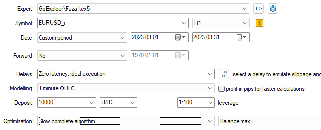
The EA will be optimized for one parameter – Start. It is used to determine the number of running agents. At the initial stage, I launched the EA with a small number of agents. This gives us a quick pass to create an initial archive of examples.
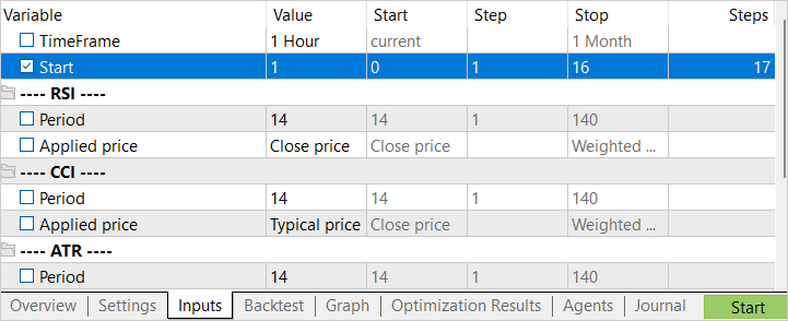
After completing the first stage of optimization, we increase the number of testing agents. Here we have 2 approaches to the next launch. If we want to try to find the best action in the most unprofitable states, then the optimization interval for the Start parameter should be indicated from "0". To select random states, we set a deliberately large initial value for parameter optimization as the starting point for the exploration. The final optimization value of the parameter depends on the number of agents being launched. The value in the Steps column corresponds to the number of agents launched during the optimization (training) process.
2.2. Second Phase: training the policy using examples
While our first EA is working to create a database of examples, we are moving on to working on the second phase EA.
In my implementation, I deviated a little from the policy training process in phase 2 proposed by the authors of the article. The article proposed the use of a simulation method to train the policy. This uses a modified approach to the reinforcement learning algorithms. In a separate section, the agent is trained to repeat the actions of a successful strategy from the examples archive, and then a standard reinforcement learning approach is applied. At the first stage, the demonstration segment of the "teacher" is maximum. The agent must obtain results no worse than the "teacher". As training progresses, the "teacher" interval decreases. The agent must learn to optimize the teacher's strategy.
In my implementation, I divided this phase into 2 stages. In the first stage, we train the agent in a similar way to the supervised learning process. However, we don't specify the correct action. Instead, we adjust the forecast reward value. For this stage, let's create the Faza2.mq5 EA.
In the EA code, we add an element describing the system state and a class of a fully parameterized FQF model.
//+------------------------------------------------------------------+
//| Includes                                                         |
//+------------------------------------------------------------------+
#include "Cell.mqh"
#include "..\RL\FQF.mqh"
//+------------------------------------------------------------------+
//| Input parameters                                                 |
//+------------------------------------------------------------------+
input int                  Iterations =  100000;
It has a minimum of external parameters. We only indicate the number of model training iterations.
Among the global parameters, we declare a model class, a state description object, and an array of rewards. We also need to declare an array to load the examples archive.
CNet                 StudyNet;
//---
float                dError;
datetime             dtStudied;
bool                 bEventStudy;
//---
CBufferFloat         State1;
CBufferFloat         *Rewards;

Cell                 Base[];
In the EA initialization method, we first upload the example archive. In this case, this is one of the key points. If there is an error loading the example archive, we will not have the source data to train the model. Therefore, in case of a loading error, we terminate the function with the INIT_FAILED result.
//+------------------------------------------------------------------+
//| Expert initialization function                                   |
//+------------------------------------------------------------------+
int OnInit()
  {
//---
   if(!LoadTotalBase())
      return(INIT_FAILED);
//---
   if(!StudyNet.Load(FileName + ".nnw", dError, dError, dError, dtStudied, true))
     {
      CArrayObj *model = new CArrayObj();
      if(!CreateDescriptions(model))
        {
         delete model;
         return INIT_FAILED;
        }
      if(!StudyNet.Create(model))
        {
         delete model;
         return INIT_FAILED;
        }
      delete model;
     }
   if(!StudyNet.TrainMode(true))
      return INIT_FAILED;
//---
   bEventStudy = EventChartCustom(ChartID(), 1, 0, 0, "Init");
//---
   return(INIT_SUCCEEDED);
  }
After loading the example archive, we initialize the model for training. As usual, we first try to load a pre-trained model. If the model fails to load for any reason, we will initialize the creation of a new model with random weights. The model description is specified in the CreateDescriptions function.
After successful model initialization, we create a custom event to start the model training process. We used the same approach for supervised learning.
Here we complete the EA's initialization function.
Please note that in this EA we did not create objects for loading historical price data and indicators. The entire learning process is based on examples. The examples archive stores all descriptions of the system state, including information about the account and open positions.
The custom event we created is processed in the OnChartEvent function. Here we only check the occurrence of the expected event and call the model training function.
//+------------------------------------------------------------------+
//| ChartEvent function                                              |
//+------------------------------------------------------------------+
void OnChartEvent(const int id,
                  const long &lparam,
                  const double &dparam,
                  const string &sparam)
  {
//---
   if(id == 1001)
      Train();
  }
The actual model training process is implemented in the Train function. This function has no parameters. In the body of the function, we first determine the size of the example archive and save the number of milliseconds from the system start in a local variable. We will use this value to periodically inform the user about the progress of the model training process.
//+------------------------------------------------------------------+
//| Train function                                                   |
//+------------------------------------------------------------------+
void Train(void)
  {
   int total = ArraySize(Base);
   uint ticks = GetTickCount();
After a little preparatory work, we organize a model training loop. The number of loop iterations corresponds to the value of the external variable. We will also provide for forced interruption of the loop and closing of the program upon user request. This can be done by the IsStopped function. If the user closes the program, the specified function will return true.
   for(int iter = 0; (iter < Iterations && !IsStopped()); iter ++)
     {
      int i = 0;
      int count = 0;
      int total_max = 0;
      i = (int)((MathRand() * MathRand() / MathPow(32767, 2)) * (total - 1));
      State1.AssignArray(Base[i].state);
      if(IsStopped())
        {
         PrintFormat("%s -> %d", __FUNCTION__, __LINE__);
         ExpertRemove();
         return;
        }
In the loop body, we randomly select one example from the archive and copy the state to the data buffer. Then we execute the feed-forward pass of the model.
      if(!StudyNet.feedForward(GetPointer(State1), 12, true))
         return;
We then retrieve the executed action in the current example, loaf the feed forward results, and update the reward for the action performed.
      int action = Base[i].total_actions;
      if(action < 0)
        {
         iter--;
         continue;
        }
      action = Base[i].actions[action];
      if(action < 0 || action > 3)
         action = 3;
      StudyNet.getResults(Rewards);
      if(!Rewards.Update(action, -Base[i].value))
         return;
Pay attention to the following two moments. If there is no action in the example (the initial state is selected), then we decrease the iteration counter and select a new example. When updating the reward, we take the value with the opposite sign. Remember? When saving the state, we made a positive value to reduce the equity. And this is a negative point.
After updating the reward, we perform a backpropagation pass and update the weights.
      if(!StudyNet.backProp(GetPointer(Rewards)))
         return;
      if(GetTickCount() - ticks > 500)
        {
         Comment(StringFormat("%.2f%% -> Error %.8f", iter * 100.0 / (double)(Iterations), StudyNet.getRecentAverageError()));
         ticks = GetTickCount();
        }
     }
At the end of the loop iterations, we check whether the learning process information needs to be updated for the user. In this example, we update the chart comment field every 0.5 seconds.
This completes the operations in the loop body, and we move on to a new example from the database.
After completing all iterations of the loop, we clear the comment field. We output the information to the log and initiate the shutdown of the EA.
   Comment("");
//---
   PrintFormat("%s -> %d -> %10.7f", __FUNCTION__, __LINE__, StudyNet.getRecentAverageError());
   ExpertRemove();
//---
  }
When closing the EA, we delete the used dynamic objects in its deinitialization method and save the trained model on disk.
//+------------------------------------------------------------------+
//| Expert deinitialization function                                 |
//+------------------------------------------------------------------+
void OnDeinit(const int reason)
  {
   if(!!Rewards)
      delete Rewards;
//---
   StudyNet.Save(FileName + ".nnw", 0, 0, 0, 0, true);
  }
After the first-phase EA collected the archive of examples, we only need to run the second-phase EA on the chart, and the model training process will begin. Please note that, unlike with the first-phase EA, we do not run the second-phase EA in the strategy tester but attach it to a real chart. In the EA parameters, we indicate the number of iterations of the learning process loop and monitor the process.
To achieve optimal results, iterations of the first and second phases can be repeated. In this case, it is possible to first repeat the first phase N times, and then repeat the second one M times. Or you can repeat the loop of first phase + second phase iterations several times.
To fine-tune the policy, we use the third EA GE-learning.mq5. It implements a classic reinforcement learning algorithm. We will not dwell in detail on all the functions of the EA now. Its full code can be found in the attachment. Let's consider only the tick processing function OnTick.
As in the first-phase EA, we only process the new candlestick opening event. If there is none, we simply complete the function while waiting for the right moment.
When the new candlestick opening event occurs, we first save the last state, the action taken and the change in equity into the experience replay buffer. And we rewrite the equity indicator into a global variable to track changes on the next candlestick.
void OnTick()
  {
   if(!IsNewBar())
      return;
//---
   float current = (float)AccountInfoDouble(ACCOUNT_EQUITY);
   if(Equity >= 0 && State1.Total() == (HistoryBars * 12 + 9))
      cReplay.AddState(GetPointer(State1), Action, (double)(current - Equity));
   Equity = current;
Then, we update the history of price values and indicators.
//---
   int bars = CopyRates(Symb.Name(), TimeFrame, iTime(Symb.Name(), TimeFrame, 1), HistoryBars, Rates);
   if(!ArraySetAsSeries(Rates, true))
     {
      PrintFormat("%s -> %d", __FUNCTION__, __LINE__);
      return;
     }
//---
   RSI.Refresh();
   CCI.Refresh();
   ATR.Refresh();
   MACD.Refresh();
Form a description of the current state of the system. Here you need to be careful to make sure that the generated description of the system state fully corresponds to a similar process in the first-phase EA. Because operation and fine-tuning should be carried out on data comparable to the data of the training sample.
   State1.Clear();
   for(int b = 0; b < (int)HistoryBars; b++)
     {
      float open = (float)Rates[b].open;
      TimeToStruct(Rates[b].time, sTime);
      float rsi = (float)RSI.Main(b);
      float cci = (float)CCI.Main(b);
      float atr = (float)ATR.Main(b);
      float macd = (float)MACD.Main(b);
      float sign = (float)MACD.Signal(b);
      if(rsi == EMPTY_VALUE || cci == EMPTY_VALUE || atr == EMPTY_VALUE || macd == EMPTY_VALUE || sign == EMPTY_VALUE)
         continue;
      //---
      if(!State1.Add((float)Rates[b].close - open) || !State1.Add((float)Rates[b].high - open) ||
         !State1.Add((float)Rates[b].low - open) || !State1.Add((float)Rates[b].tick_volume / 1000.0f) ||
         !State1.Add(sTime.hour) || !State1.Add(sTime.day_of_week) || !State1.Add(sTime.mon) ||
         !State1.Add(rsi) || !State1.Add(cci) || !State1.Add(atr) || !State1.Add(macd) || !State1.Add(sign))
        {
         PrintFormat("%s -> %d", __FUNCTION__, __LINE__);
         break;
        }
     }
//---
   if(!State1.Add((float)AccountInfoDouble(ACCOUNT_BALANCE)) || !State1.Add((float)AccountInfoDouble(ACCOUNT_EQUITY)) ||
      !State1.Add((float)AccountInfoDouble(ACCOUNT_MARGIN_FREE)) ||
      !State1.Add((float)AccountInfoDouble(ACCOUNT_MARGIN_LEVEL)) ||
      !State1.Add((float)AccountInfoDouble(ACCOUNT_PROFIT)))
      return;
//---
   double buy_value = 0, sell_value = 0, buy_profit = 0, sell_profit = 0;
   int total = PositionsTotal();
   for(int i = 0; i < total; i++)
     {
      if(PositionGetSymbol(i) != Symb.Name())
         continue;
      switch((int)PositionGetInteger(POSITION_TYPE))
        {
         case POSITION_TYPE_BUY:
            buy_value += PositionGetDouble(POSITION_VOLUME);
            buy_profit += PositionGetDouble(POSITION_PROFIT);
            break;
         case POSITION_TYPE_SELL:
            sell_value += PositionGetDouble(POSITION_VOLUME);
            sell_profit += PositionGetDouble(POSITION_PROFIT);
            return;
        }
     }
   if(!State1.Add((float)buy_value) || !State1.Add((float)sell_value) || !State1.Add((float)buy_profit) ||
      !State1.Add((float)sell_profit))
      return;
After that execute the feed-forward pass. Based on the results of the feed-forward pass, we determine and perform an action.
   if(!StudyNet.feedForward(GetPointer(State1), 12, true))
      return;
   Action = StudyNet.getAction();
   switch(Action)
     {
      case 0:
         Trade.Buy(Symb.LotsMin(), Symb.Name());
         break;
      case 1:
         Trade.Sell(Symb.LotsMin(), Symb.Name());
         break;
      case 2:
         for(int i = PositionsTotal() - 1; i >= 0; i--)
            if(PositionGetSymbol(i) == Symb.Name())
               Trade.PositionClose(PositionGetInteger(POSITION_IDENTIFIER));
         break;
     }
Please note that we do not use any exploration policy in this case. We strictly follow the learned policy.
At the end of the tick processing function, we check the time. Once a day, at midnight, we update the agent’s policy using the experience replay buffer.
   MqlDateTime time;
   TimeCurrent(time);
   if(time.hour == 0)
     {
      int repl_action;
      double repl_reward;
      for(int i = 0; i < 10; i++)
        {
         if(cReplay.GetRendomState(pstate1, repl_action, repl_reward, pstate2))
            return;
         if(!StudyNet.feedForward(pstate1, 12, true))
            return;
         StudyNet.getResults(Rewards);
         if(!Rewards.Update(repl_action, (float)repl_reward))
            return;
         if(!StudyNet.backProp(GetPointer(Rewards), DiscountFactor, pstate2, 12, true))
            return;
        }
     }
//---
  }
The full codes of all EAs can be found in the attachment.
3. Testing
All the three EAs were tested sequentially, in accordance with the Go-Explore algorithm:
- Several consecutive launches of the first-phase EA in the optimization mode of the strategy tester to create an archive of examples.
- Several iterations of policy training by the second-phase EA.
- Final fine-tuning in the strategy tester using reinforcement learning algorithms.
All tests, as in the entire series of articles, were carried out on historical data of EURUSD, timeframe H1. The indicator parameters were used by default without any adjustments.
The testing produced quite good results which are shown in the screenshots below.


Here we see a fairly even graph of balance growth. The test data reached a profit factor of 6.0 and a recovery factor of 3.34. Of the 30 performed trades, 22 were profitable, which amounted to 73.3%. The average profit of a trade is more than 2 times higher than the average loss. The maximum profit per trade is 3.5 times higher than the maximum losing trade.
Please note that the EA executed only buy trades and closed them without significant drawdowns. The reason for the absence of short trades is the topic for additional research.
The testing results are promising, but they were obtained over a short time period. To confirm the results of the algorithm, additional experiments over a longer time period are required.
Conclusion
In this article, we introduced the Go-Explore algorithm, which is a new approach to solving complex reinforcement learning problems. It is based on the idea of remembering and revisiting promising states in the state space to achieve the desired performance faster. The main difference between Go-Explore and other algorithms is its focus on finding relevant states and actions, rather than directly solving the target problem.
We have built three Expert Advisors that are run sequentially. Each of them performs its own algorithm functionality to achieve the common goal of policy learning. Policy here means the trading strategy.
The algorithm was tested using historical data and showed one of the best results. However, the results were achieved in the strategy tester over a short time period. Therefore, before using the EA on real accounts, it requires comprehensive testing and model training over a longer, more representative time period.
References
- Go-Explore: a New Approach for Hard-Exploration Problems
- Neural networks made easy (Part 35): Intrinsic Curiosity Module
- Neural networks made easy (Part 36): Relational Reinforcement Learning
- Neural networks made easy (Part 37): Sparse Attention
- Neural networks made easy (Part 38): Self-Supervised Exploration via Disagreement
Programs used in the article
| # | Issued to | Type | Description |
|---|---|---|---|
| 1 | Faza1.mq5 | Expert Advisor | First-phase Expert Advisor |
| 2 | Faza2.mql5 | Expert Advisor | Second-phase Expert Advisor |
| 3 | GE-lerning.mq5 | Expert Advisor | Policy fine-tuning Expert Advisor |
| 4 | Cell.mqh | Class library | Structure of the system state description |
| 5 | FQF.mqh | Class library | Class library for organizing the work of a fully parameterized model |
| 6 | NeuroNet.mqh | Class library | A library of classes for creating a neural network |
| 7 | NeuroNet.cl | Code Base | OpenCL program code library |
Translated from Russian by MetaQuotes Ltd.
Original article: https://www.mql5.com/ru/articles/12558
Warning: All rights to these materials are reserved by MetaQuotes Ltd. Copying or reprinting of these materials in whole or in part is prohibited.
This article was written by a user of the site and reflects their personal views. MetaQuotes Ltd is not responsible for the accuracy of the information presented, nor for any consequences resulting from the use of the solutions, strategies or recommendations described.

- Free trading apps
- Over 8,000 signals for copying
- Economic news for exploring financial markets
You agree to website policy and terms of use
I got this error.
2023.05.07 20:04:44.281 Core 01 pass 359 tested with error "critical runtime error 502 in OnTester function(array out of range, module Experts\GoExploer\Faza1.ex5, file Faza1.mq5, line 223, col 12)" in 0:00:00.202
//--- copy cell
actions[action_count] = act;
Base[action_count].total_actions = action_count+StartCell.total_actions;
how to solve it?
If the error is constantly growing, try to reduce the training coefficient.
I got this error.
2023.05.07 20:04:44.281 Core 01 pass 359 tested with error "critical runtime error 502 in OnTester function (array out of range, module Experts\GoExploer\Faza1.ex5, file Faza1.mq5, line 223, col 12)" in 0:00:00.202
//--- copy cell
actions[action_count] = act;
Base[action_count].total_actions = action_count+StartCell.total_actions;
how to solve it?
What's period of study?
What's the period of study?
H1 data, from 1 Apr 2023~ 30 Apr 2023