
Neural networks made easy (Part 49): Soft Actor-Critic

Introduction
We continue our acquaintance with algorithms for solving problems using reinforcement learning in a continuous action space. In the previous articles, we have considered the Deep Deterministic Policy Gradient (DDPG) and Twin Delayed Deep Deterministic policy gradient (TD3) algorithms. In this article, we will focus our attention on another algorithm - Soft Actor-Critic (SAC). It was first presented in the article "Soft Actor-Critic: Off-Policy Maximum Entropy Deep Reinforcement Learning with a Stochastic Actor" (January 2018). The method was presented almost simultaneously with TD3. It has some similarities, but there are also differences in the algorithms. The main goal of SAC is to maximize the expected reward given the maximum entropy of the policy, which allows finding a variety of optimal solutions in stochastic environments.
1. Soft Actor-Critic algorithm
While considering the SAC algorithm, we should probably immediately note that it is not a direct descendant of the TD3 method (and vice versa). But they have some similarities. In particular:
- they are both off-policy algorithms
- they both exploit DDPG methods
- they both use 2 Critics.
But unlike the two previously discussed methods, SAC uses a stochastic Actor policy. This allows the algorithm to explore different strategies and find optimal solutions, taking into account the maximum variety of actor actions.
Speaking about the stochasticity of the environment, we understand that in S state when performing the A action, we get the R reward within [Rmin, Rmax] with the probability of Psa.
Soft Actor-Critic uses an Actor with the stochastic policy. This means that the Actor in S state is able to choose the A' action from the entire action space with a certain Pa' probability. In other words, the Actor’s policy in each specific state allows us to choose not one specific optimal action, but any of the possible actions (but with a certain degree of probability). During the training, the Actor learns this probabilistic distribution of obtaining the maximum reward.
This property of a stochastic Actor policy allows us to explore different strategies and discover optimal solutions that may be hidden when using a deterministic policy. In addition, the stochastic Actor policy takes into account the uncertainty in the environment. In case of a noise or random factors, such policies can be more resilient and adaptive, since they can generate a variety of actions to effectively interact with the environment.
However, training the actor’s stochastic policy also makes adjustments to training. Classical reinforcement learning aims to maximize expected returns. During training, for each S action we select the A* action, which is most likely to give us greater profitability. This deterministic approach builds a clear relationship St → At → St+1 ⇒ R and leaves no room for stochastic actions. To train a stochastic policy, the authors of the Soft Actor-Critic algorithm introduce entropy regularization into the reward function.
![]()
The entropy (H) in this context is a measure of policy uncertainty or diversity. The ɑ>0 parameter is a temperature coefficient allowing us to balance between studying the environment and operating the model.
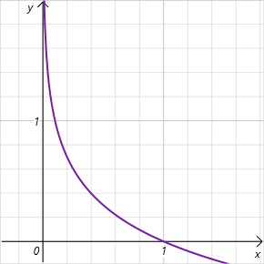
As you know, the entropy is a measure of the uncertainty of a random variable and is determined by the equation
![]()
Note that we are talking about the logarithm of the probability of choosing an action over the range of [0, 1]. In this interval of acceptable values, the graph of the entropy function is decreasing and lies in the area of positive values. Thus, the lower the probability of choosing an action, the higher the reward and the model is encouraged to explore the environment.
As you can see, in this regard, quite high requirements are put forward for the selection of the ɑ hyperparameter. Currently, there are various options for implementing the SAC algorithm. The conventional fixed parameter approach is among us. Quite often we can find implementations with a gradual decrease in the parameter. It is easy to see that when ɑ=0 we arrive at deterministic reinforcement learning. In addition, there are various approaches to optimizing the ɑ parameter by the model itself during training.
Let's move on to training the Critic. Similar to TD3, SAC trains 2 Critic models in parallel using MSE as the loss function. For the predicted value of the future state, the smaller value from the two Critic target models is used. But there are 2 key differences here.
The first one is the reward function discussed above. We use entropy regularization for both the current and subsequent states considering the discount factor applied to the cost of the next state of the system.
The second difference is the Actor. SAC does not use a target Actor model. To select an action in the current and subsequent states, one trained Actor model is used. Thus, we emphasize that reaching future rewards is achieved using current policies. In addition, using a single Actor model reduces the cost of memory and computing resources.
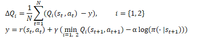
To train the Actor policy, we use DDPG approaches. We obtain the action error gradient by backpropagating the error gradient of the predicted action cost through the Critic model. But unlike TD3 (where we used only the Critic 1 model), the authors of SAC suggest using a model with a lower estimated cost of action.
There is one more thing here. During training, we change the policy, which leads to a change in the actions of the Actor in a particular state of the system. In addition, the use of a stochastic Actor policy also contributes to the variety of Actor actions. At the same time, we train models on data from the experience replay buffer with rewards for other agent actions. In this case, we are guided by the theoretical assumption that in the process of training the Actor we move in the direction of maximizing the predicted reward. This means that in any S state, the action cost using πnew new policy is not less than the action cost in the πold policy.
![]()
It is a pretty a subjective assumption, but it is fully consistent with our model training paradigm. In order not to accumulate possible errors, I can recommend updating the experience playback buffer more often during training considering updates to the Actor policy.
The updating of the target models is smoothed using the τ factor similar to TD3.
There is yet one more difference from the TD3 method. The Soft Actor-Critic algorithm does not use delay in Actor training and updating target models. Here, all models are updated at each training step.
Let's summarize the Soft Actor-Critic algorithm:
- Entropy regularization is introduced into the reward function.
- At the beginning of training, the Actor and 2 Critic models are initialized with random parameters.
- As a result of interaction with the environment, the experience replay buffer is filled in. We keep the state of the environment, the action, the subsequent state and the reward intact.
- After filling in the experience replay buffer, we train the model
- We randomly extract a set of data from the experience replay buffer
- Determine the action for the future state taking into account the current policy of the Actor
- Determine the predicted value of the future state using the current policy of at least 2 target Critics models
- Update Critics models
- Update Actor policy
- Update target models.
The process of training models is iterative and is repeated until the desired result is obtained or the minimum extremum is reached on the Critics loss function graph.
2. Implementation using MQL5
After a theoretical introduction to the Soft Actor-Critic algorithm, we move on to its implementation using MQL5. The first thing we are faced with is determining the probability of a particular action. Actually, this is quite a simple question for a tabular implementation of the Actor policy. But it causes difficulties when using neural networks. After all, we do not keep statistics on environmental conditions and actions performed. It is "hardwired" into the customizable parameters of our model. In this regard, I remembered about distributed Q-training. As you might remember, we talked about studying the probability distribution of expected reward. Distributive Q-learning allowed us to obtain a probability distribution for a given number of fixed interval reward values. The fully parameterized Q-function (FQF) model allows us to study both interval values and their probabilities.
2.1 Creating a new neural layer class
Inheriting from the CNeuronFQF class, we will create a new neural layer class to implement the proposed CNeuronSoftActorCritic algorithm. The set of methods of the new class is quite standard, but it also has its own peculiarities.
In particular, in our implementation we decided to use custom entropy regularization parameters. For this purpose, the cAlphas neural layer was added. This implementation uses the layer of the CNeuronConcatenate type. In order to decide on the size of the ratios, we will use embedding of the current state and quantile distribution at the output.
In addition, we added a separate buffer to record entropy values, which we will later use in the reward function.
Both added objects are declared static, which allows us to leave the class constructor and destructor empty.
class CNeuronSoftActorCritic  :  public CNeuronFQF
  {
protected:
   CNeuronConcatenate   cAlphas;
   CBufferFloat         cLogProbs;

   virtual bool      feedForward(CNeuronBaseOCL *NeuronOCL) override;
   virtual bool      updateInputWeights(CNeuronBaseOCL *NeuronOCL) override;

public:
                     CNeuronSoftActorCritic(void) {};
                    ~CNeuronSoftActorCritic(void) {};
   //---
   virtual bool      Init(uint numOutputs, uint myIndex, COpenCLMy *open_cl, uint actions, uint quantiles,
                          uint numInputs, ENUM_OPTIMIZATION optimization_type, uint batch);
   virtual bool      calcAlphaGradients(CNeuronBaseOCL *NeuronOCL);
   virtual bool      GetAlphaLogProbs(vector<float> &log_probs)       { return (cLogProbs.GetData(log_probs) > 0); }
   virtual bool      CalcLogProbs(CBufferFloat *buffer);
   //---
   virtual bool      Save(int const file_handle) override;
   virtual bool      Load(int const file_handle) override;
   //---
   virtual int       Type(void) override        const                 {  return defNeuronSoftActorCritic;          }
   virtual void      SetOpenCL(COpenCLMy *obj);
  };
First we will look at the Init class initialization method. The method parameters completely repeat the parameters of a similar method of the parent class. We immediately call the method of the parent class in the method body. We use this technique quite often since all the necessary controls are implemented in the parent class. The initialization of all inherited objects is carried out as well. One check of the results of the parent class method replaces full control of the mentioned operations. All we have to do is initialize the added objects.
First, we initialize the ɑ ratio calculation layer. As mentioned above, we will submit an embedding of the current state to the input of this model, the size of which will be equal to the size of the previous neural layer. Besides, we will add a quantile distribution to the output of the current layer, which will be contained in the internal layer cQuantile2 (declared and initialized in the parent class). At the output of the cAlphas layer, we are to obtain temperature coefficients for each individual action. Accordingly, the size of the layer will be equal to the number of actions.
The coefficients should be non-negative. To satisfy this requirement, we defined Sigmoid as the activation function of this layer.
At the end of the method, we initialize the entropy buffer with zero values. Its size is also equal to the number of actions. Create the buffer in the current OpenCL context right away.
bool CNeuronSoftActorCritic::Init(uint numOutputs, uint myIndex, COpenCLMy *open_cl,
                                  uint actions, uint quantiles, uint numInputs,
                                  ENUM_OPTIMIZATION optimization_type, uint batch)
  {
   if(!CNeuronFQF::Init(numOutputs, myIndex, open_cl, actions, quantiles, numInputs, optimization_type, batch))
      return false;
//---
   if(!cAlphas.Init(0, 0, OpenCL, actions, numInputs, cQuantile2.Neurons(), optimization_type, batch))
      return false;
   cAlphas.SetActivationFunction(SIGMOID);
//---
   if(!cLogProbs.BufferInit(actions, 0) || !cLogProbs.BufferCreate(OpenCL))
      return false;
//---
   return true;
  }
Next, we move on to implementing the forward pass. Here we borrow the process of training quantiles and probability distributions from the parent class without changes. But we have to add arranging the process of determining temperature coefficients and calculating entropy values. Moreover, while the calculation of the temperature involves calling a direct pass through the cAlphas layer, determining the entropy values should be implemented from "0".
We have to calculate entropy for each action of the Actor. At this stage, we expect that there will not be a lot of action here. Since all the source data is in the OpenCL context memory, it is logical to transfer our operations to this environment. First, we will create the SAC_AlphaLogProbs OpenCL kernel of the program to implement this functionality.
In the kernel parameters, we will pass 5 data buffers and 2 constants:
- outputs — results buffer contains probability-weighted sums of quantile values for each action
- quantiles — average quantile values (cQuantile2 inner layer results buffer)
- probs — probability tensor (cSoftMax inner layer results buffer)
- alphas — vector of temperature coefficients
- log_probs — vector of entropy values (in this case, the buffer for recording results)
- count_quants — number of quantiles for each action
- activation — activation function type.
The CNeuronFQF class does not use the activation function at the output. I would even say that it contradicts the very idea behind the class. After all, the distribution of average values of quantiles of the expected reward is delimited by the actual reward itself during the model training. In our case, we expect a certain value of the Actor’s action from a continuous distribution at the output of the layer. Due to various technical or other circumstances, the scope of permissible actions of an agent may be limited. The activation function allows us to do this. But it is very important for us to obtain a true probability estimate that the activation function is applied after determining the probability of the actual action. Therefore, we added its implementation to this kernel.
__kernel void SAC_AlphaLogProbs(__global float *outputs,
                                __global float *quantiles,
                                __global float *probs,
                                __global float *alphas,
                                __global float *log_probs,
                                const int count_quants,
                                const int activation
                               )
  {
   const int i = get_global_id(0);
   int shift = i * count_quants;
   float quant1 = -1e37f;
   float quant2 = 1e37f;
   float prob1 = 0;
   float prob2 = 0;
   float value = outputs[i];
We identify the current flow of operations in the kernel body. It will show us the serial number of the action being analyzed. Then we will determine the shift in the quantile and probability buffers.
Next we will declare the local variables. To determine the probability of a particular action, we need to find the 2 closest quantiles. In the quant1 variable, we will write the average value of the lowest quantile. The quant2 variable will contain the average value of the quantile closest to the top. At the initial stage, we initialize the specified variables with obviously extreme values. We will store the corresponding probabilities in the prob1 and prob2 variables, which we will initialize with zero values. Indeed, in our understanding, the probability of obtaining such extreme values is “0”.
We will save the desired value from the buffer into the local variable value.
Due to the specific memory organization of the OpenCL context, accessing local variables is many times faster than retrieving data from the global memory buffer. Operating with local variables, we increase the performance of the entire OpenCL program.
Now that we have stored the desired value in a local variable, we can painlessly apply the activation function to the buffer of the neural layer operation results.
   switch(activation)
     {
      case 0:
         outputs[i] = tanh(value);
         break;
      case 1:
         outputs[i] = 1 / (1 + exp(-value));
         break;
      case 2:
         if(value < 0)
            outputs[i] = value * 0.01f;
         break;
      default:
         break;
     }
Next, we arrange the cycle of searching through all the average quantile values and looking for the closest ones.
It should be noted here that we did not sort the average quantile values. The weighted average determinations are not affected by this, and we have previously avoided performing unnecessary operations. Therefore, with a high degree of probability, the quantiles closest to the desired value will not be located in neighboring elements of the quantile buffer. Therefore, we iterate over all values.
In order not to write the values of the same quantile into both variables, we use the logical operator “>=" for the lower bound, and strictly “<” for the upper bound. When a quantile is closer to the previously stored one, we rewrite the value in the previously declared corresponding variables to quantile mean value and its probability.
   for(int q = 0; q < count_quants; q++)
     {
      float quant = quantiles[shift + q];
      if(value >= quant && quant1 < quant)
        {
         quant1 = quant;
         prob1 = probs[shift + q];
        }
      if(value < quant && quant2 > quant)
        {
         quant2 = quant;
         prob2 = probs[shift + q];
        }
     }
After completing all iterations of the loop, our local variables will contain the data of the nearest quantiles. The necessary value is somewhere within that range. However, our knowledge of the probability distribution of actions is limited only by the studied distribution. In this case, we use the assumption of a linear dependence of the probability between the 2 nearest quantiles. With a sufficiently large number of quantiles, taking into account the limited range of distribution of values of the actual actions area, our assumption is not far from the truth.
   float prob = fabs(value - quant1) / fabs(quant2 - quant1);
   prob = clamp((1-prob) * prob1 + prob * prob2, 1.0e-3f, 1.0f);
   log_probs[i] = -alphas[i] * log(prob);
  }
After determining the action probability, we determine the entropy of the action and multiply the resulting value by the temperature coefficient. To avoid too high entropy values, I limited the lower bound of the probability to 0.001.
Now let's move on to the main program. Here we create a forward pass method for our CNeuronSoftActorCritic::feedForward class.
As you remember, here we widely exploit the capabilities of virtual methods in inherited objects. Therefore, the method parameters completely repeat similar methods of all previously discussed classes.
In the method body, we first call the forward pass method of the parent class and a similar layer method for calculating temperature coefficients. Here we just need to check the results of executing these methods.
bool CNeuronSoftActorCritic::feedForward(CNeuronBaseOCL *NeuronOCL)
  {
   if(!CNeuronFQF::feedForward(NeuronOCL))
      return false;
   if(!cAlphas.FeedForward(GetPointer(cQuantile0), cQuantile2.getOutput()))
      return false;
Next we have to calculate the entropy component of the reward function. To do this, we arrange the process of launching the kernel discussed above. We will run it in a one-dimensional task space according to the number of actions being analyzed.
   uint global_work_offset[1] = {0};
   uint global_work_size[1] = {Neurons()};
As always, before placing the kernel in the execution queue, we pass the initial data to its parameters.
   if(!OpenCL.SetArgumentBuffer(def_k_SAC_AlphaLogProbs, def_k_sac_alp_alphas, cAlphas.getOutputIndex()))
     {
      printf("Error of set parameter kernel %s: %d; line %d", __FUNCTION__, GetLastError(), __LINE__);
      return false;
     }
   if(!OpenCL.SetArgumentBuffer(def_k_SAC_AlphaLogProbs, def_k_sac_alp_log_probs, cLogProbs.GetIndex()))
     {
      printf("Error of set parameter kernel %s: %d; line %d", __FUNCTION__, GetLastError(), __LINE__);
      return false;
     }
   if(!OpenCL.SetArgumentBuffer(def_k_SAC_AlphaLogProbs, def_k_sac_alp_outputs, getOutputIndex()))
     {
      printf("Error of set parameter kernel %s: %d; line %d", __FUNCTION__, GetLastError(), __LINE__);
      return false;
     }
   if(!OpenCL.SetArgumentBuffer(def_k_SAC_AlphaLogProbs, def_k_sac_alp_probs, cSoftMax.getOutputIndex()))
     {
      printf("Error of set parameter kernel %s: %d; line %d", __FUNCTION__, GetLastError(), __LINE__);
      return false;
     }
   if(!OpenCL.SetArgumentBuffer(def_k_SAC_AlphaLogProbs, def_k_sac_alp_quantiles, cQuantile2.getOutputIndex()))
     {
      printf("Error of set parameter kernel %s: %d; line %d", __FUNCTION__, GetLastError(), __LINE__);
      return false;
     }
   if(!OpenCL.SetArgument(def_k_SAC_AlphaLogProbs, def_k_sac_alp_count_quants, (int)(cSoftMax.Neurons() / global_work_size[0])))
     {
      printf("Error of set parameter kernel %s: %d; line %d", __FUNCTION__, GetLastError(), __LINE__);
      return false;
     }
   if(!OpenCL.SetArgument(def_k_SAC_AlphaLogProbs, def_k_sac_alp_activation, (int)activation))
     {
      printf("Error of set parameter kernel %s: %d; line %d", __FUNCTION__, GetLastError(), __LINE__);
      return false;
     }
Please note that we are not checking any buffers. The fact is that all used buffers have already been checked at the stage of direct pass of the parent class method and the layer for calculating temperature ratios. The only thing remaining unchecked has been the internal buffer for recording the results of the kernel operation. But this is an internal object. Its creation was controlled at the initialization stage of the class object. There is no access to the object from an external program. The probability of getting an error here is quite low. Therefore, we take such a risk to speed up our program.
At the end of the method, we place the kernel in the execution queue and check the result of the operations.
   if(!OpenCL.Execute(def_k_SAC_AlphaLogProbs, 1, global_work_offset, global_work_size))
     {
      printf("Error of execution kernel %s: %d", __FUNCTION__, GetLastError());
      return false;
     }
//---
   return true;
  }
I would like to point out once again that in this case we are checking the result of placing the kernel in the execution queue, but not the results of executing operations inside the kernel. To obtain the results, we will need to load the cLogProbs buffer data into the main memory. This functionality is implemented in the GetAlphaLogProbs method. The method code fits in one string and is provided in the class structure description block.
Let’s move on to creating the reverse pass functionality. The main part of the functionality is already implemented in the method of the parent class. Strange as it may seem, we will not even redefine the method of distributing the error gradient through the neural layer. The fact is that the distribution of the error gradient for entropy regularization does not fully fit into our general structure. We get the error gradient by action from the last layer of the Critic model. We included the entropy regularization itself in the reward function. Accordingly, its error will also be at the level of reward prediction, i.e. at the level of the Critic results layer. Here we get 2 questions:
- The introduction of an additional gradient buffer will disrupt the virtualization model of the reverse pass methods.
- At the stage of the Actor's reverse pass, we simply do not have data about the Critic's error. It is necessary to build a new process for the entire model.
To simplify things, I have created a new parallel process only for the gradient of the entropy regularization error without completely revising the backpropagation process in the model.
First, we will create a kernel in the OpenCL program. Its code is pretty simple. We just multiply the resulting error gradient by the entropy. Then we adjust the resulting value by the derivative of the activation function of the layer for calculating the temperature ratios.
__kernel void SAC_AlphaGradients(__global float *outputs,
                                 __global float *gradient,
                                 __global float *log_probs,
                                 __global float *alphas_grad,
                                 const int activation
                                )
  {
   const int i = get_global_id(0);
   float out = outputs[i];
//---
   float grad = -gradient[i] * log_probs[i];
   switch(activation)
     {
      case 0:
         out = clamp(out, -1.0f, 1.0f);
         grad = clamp(grad + out, -1.0f, 1.0f) - out;
         grad = grad * max(1 - pow(out, 2), 1.0e-4f);
         break;
      case 1:
         out = clamp(out, 0.0f, 1.0f);
         grad = clamp(grad + out, 0.0f, 1.0f) - out;
         grad = grad * max(out * (1 - out), 1.0e-4f);
         break;
      case 2:
         if(out < 0)
            grad = grad * 0.01f;
         break;
      default:
         break;
     }
//---
   alphas_grad[i] = grad;
  }
Here we should note that to simplify the calculations, we simply multiply the gradient by the value from the log_probs buffer. As you remember, during the forward passage, we set the entropy value here taking into account the temperature ratio. From the mathematical point of view, we need to divide the value from the buffer by this value. But for the temperature we use sigmoid as the activation function. Therefore, its value is always in the range [0,1]. Dividing by a positive number less than 1 will only increase the error gradient. In this case, we deliberately do not do this.
After finishing work on the SAC_AlphaGradients kernel, we will move on to working on the main program and create the CNeuronSoftActorCritic::calcAlphaGradients method. At this stage, we will first put the kernel in the execution queue calling the methods of internal objects afterwards. Therefore, we arrange a control unit before starting the process.
bool CNeuronSoftActorCritic::calcAlphaGradients(CNeuronBaseOCL *NeuronOCL)
  {
   if(!OpenCL || !NeuronOCL || !NeuronOCL.getGradient() ||
      !NeuronOCL.getGradientIndex()<0)
      return false;
Next, we define the kernel's task space and pass the input data to its parameters.
   uint global_work_offset[1] = {0};
   uint global_work_size[1] = {Neurons()};
   if(!OpenCL.SetArgumentBuffer(def_k_SAC_AlphaGradients, def_k_sac_alg_outputs, cAlphas.getOutputIndex()))
     {
      printf("Error of set parameter kernel %s: %d; line %d", __FUNCTION__, GetLastError(), __LINE__);
      return false;
     }
   if(!OpenCL.SetArgumentBuffer(def_k_SAC_AlphaGradients, def_k_sac_alg_alphas_grad, cAlphas.getGradientIndex()))
     {
      printf("Error of set parameter kernel %s: %d; line %d", __FUNCTION__, GetLastError(), __LINE__);
      return false;
     }
   if(!OpenCL.SetArgumentBuffer(def_k_SAC_AlphaGradients, def_k_sac_alg_gradient, NeuronOCL.getGradientIndex()))
     {
      printf("Error of set parameter kernel %s: %d; line %d", __FUNCTION__, GetLastError(), __LINE__);
      return false;
     }
   if(!OpenCL.SetArgumentBuffer(def_k_SAC_AlphaGradients, def_k_sac_alg_log_probs, cLogProbs.GetIndex()))
     {
      printf("Error of set parameter kernel %s: %d; line %d", __FUNCTION__, GetLastError(), __LINE__);
      return false;
     }
   if(!OpenCL.SetArgument(def_k_SAC_AlphaGradients, def_k_sac_alg_activation, (int)cAlphas.Activation()))
     {
      printf("Error of set parameter kernel %s: %d; line %d", __FUNCTION__, GetLastError(), __LINE__);
      return false;
     }
After that, we put the kernel into the execution queue and monitor the execution of operations.
   if(!OpenCL.Execute(def_k_SAC_AlphaGradients, 1, global_work_offset, global_work_size))
     {
      printf("Error of execution kernel %s: %d", __FUNCTION__, GetLastError());
      return false;
     }
At the end of the method, we call the reverse pass method of our inner temperature coefficient calculation layer.
   return cAlphas.calcHiddenGradients(GetPointer(cQuantile0), cQuantile2.getOutput(), cQuantile2.getGradient());
  }
In addition, we will override the method for updating the parameters of the CNeuronSoftActorCritic::updateInputWeights neural layer. The method algorithm is quite simple. It only calls similar methods of the parent class and internal objects. Find the complete code of this method in the attachment. There you will also find the complete code of all methods and classes used in the article including methods for working with files of our new class, which I will not dwell on now.
2.2 Making changes to the CNet class
After completing the new class, we declare constants for servicing the created kernels. We should also add new kernels to the initialization process of the context object and the OpenCL program. I have considered this functionality more than 50 times when creating each new kernel, so I will not dwell on it.
Our library functionality does not allow a user to directly access a specific neural layer. The entire interaction process is built through the functionality of the model as a whole at the CNet class level. In order to obtain the values of the entropy component, we will create the CNet::GetLogProbs method.
In the parameters, the method receives the pointer to the vector for setting values.
In the method body, we arrange a block of controls with a step-by-step reduction in the level of objects. First, we check for the presence of a dynamic array object of neural layers. Then we go down one level and check the pointer to the object of the last neural layer. Next, we go even lower and check the type of the last neural layer. This should be our new CNeuronSoftActorCritic layer.
bool CNet::GetLogProbs(vectorf &log_probs)
  {
//---
   if(!layers)
      return false;
   int total = layers.Total();
   if(total <= 0 || !layers.At(total - 1))
      return false;
   CLayer *layer = layers.At(total - 1);
   if(!layer.At(0) || layer.At(0).Type() != defNeuronSoftActorCritic)
      return false;
//---
   CNeuronSoftActorCritic *neuron = layer.At(0);
Only after successfully passing all levels of control do we turn to a similar method of our neural layer.
   return neuron.GetAlphaLogProbs(log_probs);
  }
Please note that we are limited to only the last layer in the model at this stage. This implies that the layer can only be used as the final layer of an Actor.
Besides, the method only reads data from the buffer and does not launch their calculation. Therefore, calling it makes sense only after the direct passage of the Actor. In fact, this is not a limitation. Indeed, entropy regularization will be used only to form a reward while collecting primary data and training models. In these processes, the forward pass of the Actor with the generation of action to execution is primary.
For the needs of the reverse pass, we will create the CNet::AlphasGradient method. As we said above, the distribution of the gradient by entropy goes beyond the scope of the process we previously built. This is reflected in the method algorithm as well. We have constructed the method in such a way that we will call it for the Critic. In the method parameters, we will pass the pointer to the Actor object.
The algorithm of the control unit of this method is built accordingly. First, we check that the pointer to the Actor object is up to date and that it contains the latest CNeuronSoftActorCritic layer.
bool CNet::AlphasGradient(CNet *PolicyNet)
  {
   if(!PolicyNet || !PolicyNet.layers)
      return false;
   int total = PolicyNet.layers.Total();
   if(total <= 0)
      return false;
   CLayer *layer = PolicyNet.layers.At(total - 1);
   if(!layer || !layer.At(0))
      return false;
   if(layer.At(0).Type() != defNeuronSoftActorCritic)
      return true;
//---
   CNeuronSoftActorCritic *neuron = layer.At(0);
The second part of the control block carries out similar checks for the last Critic layer. Here there is no restriction on the type of a neural layer.
   if(!layers)
      return false;
   total = layers.Total();
   if(total <= 0 || !layers.At(total - 1))
      return false;
   layer = layers.At(total - 1);
After successfully passing all the controls, we turn to the method of distributing the gradient of our new neural layer.
   return neuron.calcAlphaGradients((CNeuronBaseOCL*) layer.At(0));
  }
To be fair, using a fully parameterized model allows us to determine the probabilities of individual actions. But it does not allow creating a truly stochastic Actor policy. Actor stochasticity involves sampling actions from a learned distribution, which we cannot do on the OpenCL context side. In the variational auto encoder, to solve a similar problem, we used a trick with reparameterization and a vector of random values generated on the side of the main program. But in this case, we will need to load the probability distribution for sampling. Instead, at the stage of collecting a database of examples, we will sample values in some environment of the calculated value (by analogy with TD3) and then ask the model for the entropy of such actions. For these purposes, we will create the CNet::CalcLogProbs method. Its algorithm is similar to the construction of the GetLogProbs method, but unlike the previous one, in the parameters we will receive a pointer to the data buffer with sampled values. As a result of the method operations in the same buffer, we will receive their probabilities.
The full code of all classes and their methods is available in the attachment.
2.3 Creating model training EAs
After completing work on creating new objects for our model, we move on to arranging the process of its creation and training. As before, will use 3 EAs:
- Research — collecting examples database
- Study — model training
- Test — checking obtained results.
In order to reduce the length of the article and save your time, I will focus only on the changes made to the versions of similar advisors from the previous article to arrange the algorithm in question.
First of all, the model architecture. Here we only changed the last Actor layer, replacing it with the new CNeuronSoftActorCritic class. We specified the layer size by the number of actions and 32 quantiles for each action (as recommended by the authors of the FQF method).
We used the sigmoid as the activation function, similar to the experiments in the previous article.
bool CreateDescriptions(CArrayObj *actor, CArrayObj *critic)
  {
//--- Actor
.........
.........
//--- layer 9
   if(!(descr = new CLayerDescription()))
      return false;
   descr.type = defNeuronSoftActorCritic;
   descr.count = NActions;
   descr.window_out = 32;
   descr.optimization = ADAM;
   descr.activation = SIGMOID;
   if(!actor.Add(descr))
     {
      delete descr;
      return false;
     }
//--- Critic
.........
.........
//---
   return true;
  }
The "...\SoftActorCritic\Research.mq5" EA algorithm has been transferred from the previous article with almost no changes. Neither the historical data collection block nor the trading operations block has undergone any changes. Changes were made only to the OnTick function in terms of environmental rewards. As mentioned above, the Soft Actor-Critic algorithm adds entropy regularization to the reward function.
As before, we use the relative change in the account balance as compensation. We also add a penalty for the lack of open positions. But next we need to add entropy regularization. I have created the above mentioned CalcLogProbs method for this. But there is one caveat. The quantile distribution of our class stores the values up to the activation function. In the decision-making process, we use the activated results of the Actor model. We use a sigmoid as the activation function at the output of the Actor.
![]()
Through mathematical transformations, we arrive at
![]()
Let's use this property and adjust the sampled actions to the required form. Then we will transfer the data from the vector to the data buffer and, if possible, transfer the information to the OpenCL context memory.
After completing such preparatory work, we ask the Actor for the entropy of the actions performed.
Note that we got the entropy of 6 actions taking into account the temperature ratio. But our reward is one number to evaluate the entirety of the current state and action. In this implementation, we used the total entropy value, which fits well into the context of probabilities and logarithms since the probability of a complex event is equal to the product of the probabilities of its component events. And the logarithm of the product is equal to the sum of the logarithms of the individual factors. However, there may be other approaches as well. Their appropriateness for each individual case can be checked during training. Do not be afraid to experiment.
void OnTick()
  {
//---
.........
.........
//---
   float reward = Account[0];
   if((buy_value + sell_value) == 0)
      reward -= (float)(atr / PrevBalance);
   for(ulong i = 0; i < temp.Size(); i++)
      sState.action[i] = temp[i];
   temp.Clip(0.001f, 0.999f);
   temp = MathLog((temp - 1.0f) * (-1.0f) / temp) * (-1);
   Result.AssignArray(temp);
   if(Result.GetIndex() >= 0)
      Result.BufferWrite();
   if(Actor.CalcLogProbs(Result))
     {
      Result.GetData(temp);
      reward += temp.Sum();
     }
   if(!Base.Add(sState, reward))
      ExpertRemove();
  }
The most significant changes were made to the model training in the "...\SoftActorCritic\Study.mq5" EA. Let's take a closer look at the Train function of the specified EA. This is where the entire model training process is arranged.
At the beginning of the function, we sample a set of data from the experience replay buffer, as we did before.
void Train(void)
  {
   int total_tr = ArraySize(Buffer);
   uint ticks = GetTickCount();
//---
   for(int iter = 0; (iter < Iterations && !IsStopped()); iter ++)
     {
      int tr = (int)((MathRand() / 32767.0) * (total_tr - 1));
      int i = (int)((MathRand() * MathRand() / MathPow(32767, 2)) * (Buffer[tr].Total - 2));
Next, we determine the predicted value of the future state. The algorithm repeats a similar process in the implementation of the TD3 method. The only difference is the absence of a target Actor model. Here, we use a trainable Actor model to determine the action in the future state.
      //--- Target
      State.AssignArray(Buffer[tr].States[i + 1].state);
      float PrevBalance = Buffer[tr].States[i].account[0];
      float PrevEquity = Buffer[tr].States[i].account[1];
      Account.Clear();
      Account.Add((Buffer[tr].States[i + 1].account[0] - PrevBalance) / PrevBalance);
      Account.Add(Buffer[tr].States[i + 1].account[1] / PrevBalance);
      Account.Add((Buffer[tr].States[i + 1].account[1] - PrevEquity) / PrevEquity);
      Account.Add(Buffer[tr].States[i + 1].account[2]);
      Account.Add(Buffer[tr].States[i + 1].account[3]);
      Account.Add(Buffer[tr].States[i + 1].account[4] / PrevBalance);
      Account.Add(Buffer[tr].States[i + 1].account[5] / PrevBalance);
      Account.Add(Buffer[tr].States[i + 1].account[6] / PrevBalance);
      //---
      if(Account.GetIndex() >= 0)
         Account.BufferWrite();
Fill in the source data buffers and call the forward pass methods of the Actor and the 2 target models of the Critic.
      if(!Actor.feedForward(GetPointer(State), 1, false, GetPointer(Account)))
        {
         PrintFormat("%s -> %d", __FUNCTION__, __LINE__);
         ExpertRemove();
         break;
        }
      //---
      if(!TargetCritic1.feedForward(GetPointer(Actor), LatentLayer, GetPointer(Actor)) ||
         !TargetCritic2.feedForward(GetPointer(Actor), LatentLayer, GetPointer(Actor)))
        {
         PrintFormat("%s -> %d", __FUNCTION__, __LINE__);
         break;
        }
As in the TD3 method, we use the smallest predicted state cost value to train the Critic. But in this case we add an entropy component.
      vector<float> log_prob;
      if(!Actor.GetLogProbs(log_prob))
        {
         PrintFormat("%s -> %d", __FUNCTION__, __LINE__);
         break;
        }
      TargetCritic1.getResults(Result);
      float reward = Result[0];
      TargetCritic2.getResults(Result);
      reward = Buffer[tr].Revards[i] + DiscFactor * (MathMin(reward, Result[0]) + log_prob.Sum() - Buffer[tr].Revards[i + 1]);
It should be noted here that in the process of saving the trajectory, we saved the cumulative amount of rewards until the end of the passage taking into account the discount factor. In this case, the reward for each individual transition to a new state includes entropy regularization. To train Critic models, we adjust the stored accumulative reward to account for the use of the updated policy. To do this, we take the difference between the minimum predicted cost of the subsequent state, taking into account the entropy component and the cumulative reward experience of this state saved in the replay buffer. Adjust the resulting value by the discount factor and add it to the saved value of the current state. In this case, we use the assumption that the cost of actions does not decrease in the process of optimizing models.
Next we face the stage of training Critics models. To do this, we fill data buffers with the current state of the system.
      //--- Q-function study
      State.AssignArray(Buffer[tr].States[i].state);
      PrevBalance = Buffer[tr].States[MathMax(i - 1, 0)].account[0];
      PrevEquity = Buffer[tr].States[MathMax(i - 1, 0)].account[1];
      Account.Update(0, (Buffer[tr].States[i].account[0] - PrevBalance) / PrevBalance);
      Account.Update(1, Buffer[tr].States[i].account[1] / PrevBalance);
      Account.Update(2, (Buffer[tr].States[i].account[1] - PrevEquity) / PrevEquity);
      Account.Update(3, Buffer[tr].States[i].account[2]);
      Account.Update(4, Buffer[tr].States[i].account[3]);
      Account.Update(5, Buffer[tr].States[i].account[4] / PrevBalance);
      Account.Update(6, Buffer[tr].States[i].account[5] / PrevBalance);
      Account.Update(7, Buffer[tr].States[i].account[6] / PrevBalance);
      //---
      Account.BufferWrite();
Please note that in this case we no longer check for the presence of an account state description buffer in the OpenCL context. Immediately after saving the data, we simply call the method of transferring data to the context. This is possible due to the fact that all our models work in the same OpenCL context. We have already talked about the advantages of this approach earlier. When calling forward pass methods on target models, a buffer has already been created in the context. Otherwise, we would receive an error when executing them. Therefore, we no longer waste time and resources on unnecessary verification at this stage.
After loading the data, we call the Actor's forward pass method and load the entropy component of the reward.
      if(!Actor.feedForward(GetPointer(State), 1, false, GetPointer(Account)))
        {
         PrintFormat("%s -> %d", __FUNCTION__, __LINE__);
         break;
        }
      //---
      Actor.GetLogProbs(log_prob);
At this stage, we have all the necessary data for the forward and reverse passages of the Critics. But at this stage we made a slight deviation from the author’s algorithm. The fact is that the authors of the method, after updating the parameters of the Critics, propose using a Critic with a minimum score to update the Actor’s policy. According to our observations, despite deviations in estimates, the gradient of the error in action is practically unchanged. So I decided to simply alternate the Critics models. At even-numbered iterations, we update Critic 2 model based on actions from the experience replay buffer. We train the Actor’s policy based on the assessments of the first Critic.
      Actions.AssignArray(Buffer[tr].States[i].action);
      if(Actions.GetIndex() >= 0)
         Actions.BufferWrite();
//---
      if((iter % 2) == 0)
        {
         if(!Critic1.feedForward(GetPointer(Actor), LatentLayer, GetPointer(Actor)) ||
            !Critic2.feedForward(GetPointer(Actor), LatentLayer, GetPointer(Actions)))
           {
            PrintFormat("%s -> %d", __FUNCTION__, __LINE__);
            break;
           }
         Result.Clear();
         Result.Add(reward-log_prob.Sum());
         if(!Critic1.backProp(Result, GetPointer(Actor)) ||
            !Critic1.AlphasGradient(GetPointer(Actor)) ||
            !Actor.backPropGradient(GetPointer(Account), GetPointer(Gradient), LatentLayer) ||
            !Actor.backPropGradient(GetPointer(Account), GetPointer(Gradient)))
           {
            PrintFormat("%s -> %d", __FUNCTION__, __LINE__);
            break;
           }
         Result.Update(0,Buffer[tr].Revards[i]);
         if(!Critic2.backProp(Result, GetPointer(Actions), GetPointer(Gradient)))
           {
            PrintFormat("%s -> %d", __FUNCTION__, __LINE__);
            break;
           }
        }
Цe change the use of Critic models on odd iterations.
      else
        {
         if(!Critic2.feedForward(GetPointer(Actor), LatentLayer, GetPointer(Actor)) ||
            !Critic1.feedForward(GetPointer(Actor), LatentLayer, GetPointer(Actions)))
           {
            PrintFormat("%s -> %d", __FUNCTION__, __LINE__);
            break;
           }
         Result.Clear();
         Result.Add(reward);
         if(!Critic2.backProp(Result, GetPointer(Actor)) ||
            !Critic2.AlphasGradient(GetPointer(Actor)) ||
            !Actor.backPropGradient(GetPointer(Account), GetPointer(Gradient), LatentLayer) ||
            !Actor.backPropGradient(GetPointer(Account), GetPointer(Gradient)))
           {
            PrintFormat("%s -> %d", __FUNCTION__, __LINE__);
            break;
           }
         Result.Update(0,Buffer[tr].Revards[i]);
         if(!Critic1.backProp(Result, GetPointer(Actions), GetPointer(Gradient)))
           {
            PrintFormat("%s -> %d", __FUNCTION__, __LINE__);
            break;
           }
        }
Pay attention to the order in which the reverse pass methods are called. First we perform a reverse Critic pass. Then we pass the gradient through the entropy component. Next, we perform a reverse pass through the Actor’s primary data processing block. This allows us to tailor convolutional layers to Critic's requirements. After doing all this, we perform a complete reverse pass of the Actor to optimize the policy of its actions.
At the end of the function operations, we update the target models and display an information message to a user to visually monitor the training process.
      //--- Update Target Nets
      TargetCritic1.WeightsUpdate(GetPointer(Critic1), Tau);
      TargetCritic2.WeightsUpdate(GetPointer(Critic2), Tau);
      //---
      if(GetTickCount() - ticks > 500)
        {
         string str = StringFormat("%-15s %5.2f%% -> Error %15.8f\n", "Critic1",
                                    iter * 100.0 / (double)(Iterations), Critic1.getRecentAverageError());
         str += StringFormat("%-15s %5.2f%% -> Error %15.8f\n", "Critic2",
                                    iter * 100.0 / (double)(Iterations), Critic2.getRecentAverageError());
         Comment(str);
         ticks = GetTickCount();
        }
     }
   Comment("");
//---
   PrintFormat("%s -> %d -> %-15s %10.7f", __FUNCTION__, __LINE__, "Critic1", Critic1.getRecentAverageError());
   PrintFormat("%s -> %d -> %-15s %10.7f", __FUNCTION__, __LINE__, "Critic2", Critic2.getRecentAverageError());
   ExpertRemove();
//---
  }
The full Expert Advisor code can be found in the attachment. There you will also find the test EA code. The changes made to it are similar to the changes in the primary data collection EA, and we will not dwell on them.
3. Test
The model was trained and tested on historical data of EURUSD H1 within January - May 2023. The indicator parameters and all hyperparameters were set to their default values.
To my regret, I must admit that while working on the article, I was unable to train a model capable of generating profit on the training set. According to the test results, my model lost 3.8% over the 5-month training period.

On the positive side, the maximum profitable trade is 3.6 times higher than the maximum loss per 1 trade. The average winning trade is only slightly higher than the average losing trade. But the share of profitable trades is 49%. Essentially, this 1% was not enough to reach "0".
For data outside the training set, the situation remained almost unchanged. Even the share of profitable trades increased to 51%. But the size of the average profitable trade decreased causing a loss again.

The stability of the model outside the training set is a positive factor. But the question remains how we can get rid of losses. Perhaps, the reason lies in the algorithm changes or in inflated temperature ratio stimulating more market research.
In addition, the reason may be that the sampled action values are too scattered. When sampling an action with a probability close to "0", high entropy inflates their rewards and this distorts the Actor's policy. To find the cause, we will need additional tests. I will share their results with you.
Conclusion
In this article, we introduced the Soft Actor-Critic (SAC) algorithm designed to solve problems in a continuous action space. It is based on the idea of maximizing policy entropy, which allows the agent to explore different strategies and find optimal solutions in stochastic environments taking into account the maximum variety of actions.
The authors of the method proposed using entropy regularization, which is added to the training objective function. This allows the algorithm to encourage exploration of new actions and prevents it from becoming too rigidly fixed on certain strategies.
We implemented this method using MQL5, but, unfortunately, were unable to train a profitable strategy. However, the trained model demonstrates stable performance on and outside the training set. This indicates the ability of the method to generalize the experience gained and transfer it to unknown environmental conditions.
I have set myself the goal of searching for opportunities to train a profitable Actor policy. The results will be presented later.
List of references
- Soft Actor-Critic: Off-Policy Maximum Entropy Deep Reinforcement Learning with a Stochastic Actor
- Soft Actor-Critic Algorithms and Applications
- Neural networks made easy (Part 48): Methods for reducing overestimation of Q-function values
Programs used in the article
| # | Name | Type | Description |
|---|---|---|---|
| 1 | Research.mq5 | Expert Advisor | Example collection EA |
| 2 | Study.mq5 | Expert Advisor | Agent training EA |
| 3 | Test.mq5 | Expert Advisor | Model testing EA |
| 4 | Trajectory.mqh | Class library | System state description structure |
| 5 | NeuroNet.mqh | Class library | A library of classes for creating a neural network |
| 6 | NeuroNet.cl | Code Base | OpenCL program code library |
Translated from Russian by MetaQuotes Ltd.
Original article: https://www.mql5.com/ru/articles/12941
Warning: All rights to these materials are reserved by MetaQuotes Ltd. Copying or reprinting of these materials in whole or in part is prohibited.
This article was written by a user of the site and reflects their personal views. MetaQuotes Ltd is not responsible for the accuracy of the information presented, nor for any consequences resulting from the use of the solutions, strategies or recommendations described.

- Free trading apps
- Over 8,000 signals for copying
- Economic news for exploring financial markets
You agree to website policy and terms of use
I discovered a new NN sequence: enjoy <3
The picture can also be simply dragged into the text or pasted with Ctrl+V