Quantization in machine learning (Part 2): Data preprocessing, table selection, training CatBoost models

Introduction

The article considers the practical application of quantization in the construction of tree models No complex mathematical equations are used. This is the second part of the article "Quantization and other methods of preprocessing input data in machine learning", so I strongly recommend starting your acquaintance with it. Here we will talk about the following:

• In the first part, we will consider the methods for preprocessing sample data implemented in MQL5.
• In the second part, we will conduct an experiment that will provide information on the feasibility of data quantization.

 

1. Additional data preprocessing methods

Let's consider the data preprocessing methods I have implemented using the example of describing the functionality of the Q_Error_Selection script.

In brief, the objective of the "Q_Error_Selection" script is to load a sample from the "train.csv" file, transfer the contents into the matrix, preprocess the data, alternately load quantum tables and assess the error of the recovered data relative to the original ones for each predictor. The assessment results of each quantum table are to be saved into the array. After checking all the options, we will create a summary table with errors for each predictor and select the best options for quantum tables for each predictor according to a given criterion. Let's create and save a summary quantum table, a file with CatBoost settings, to which predictors excluded from the list for training will be added with serial numbers of their columns. Also, create accompanying files depending on the selected script settings.

Let's take a closer look at the script settings that I have listed below by group.

 

Loading data

• Sample directory¹
• Quantization directory²

¹ Indicate the path to the directory containing the Setup directory the csv files with the sample are located in. The directory will be referred to below as the "project directory".

² Indicate the path to the directory containing the Q directory the csv files with quantum tables are located in.

 

Configuring spike handling

• Use spike check¹
• Spike conversion method:²
• The spike value is converted to the value close to the split ^2.1
• The spike value is converted to a random value in the range outside the spike^2.2
• Replace data after handling spikes³
• Save/do not save the 'train' sample with transformed spikes⁴
• Add information to subsamples about spikes⁵
• Remove rows with a large number of spikes^5.1
• Maximum percentage of predictor outliers in the sample string^5.2

¹ When selecting "true", spike handling is activated. Rare values of predictors are considered spikes here. Rare values may be statistically insignificant, but models typically do not take this into account, which can lead to questionable rules for estimating classification probability. The Figure 1 demonstrates such a spike. By setting boundaries separating spikes and normal data, we will be able to aggregate outliers into a single whole, due to which the statistical reliability will increase and we can try to work with the data as with normal data, or completely exclude it from training.

 ² Select one of the spike transformation methods, with the help of which the value of the predictor will be changed allowing this example to be taken into account in the training sample, and not excluded as an anomalous one. To determine the spikes, I used 2.5% of the data for each side of the number series. The previously encountered identical number values were grouped and ranks were assigned to the groups. If the next rank exceeds 2.5%, then the previous rank is considered the last rank with spikes. Predictors with few ranks are considered categorical and do not handle spikes. Information in the form of a list of categorical predictors is saved in the following path relative to the "..\CB\Categ.txt" project directory. A common method for identifying spikes is the three-sigma rule, which is when an indentation of three standard deviations is made from the average value to the left and right of the data area and everything that is outside this boundary is considered a spike. In the graphs below, you can see three horizontal lines in black - the center, the difference and the sum of three sigmas from the center. The blue lines on the graph will indicate the boundaries, within which frequently occurring data are located according to the algorithm I propose.

 

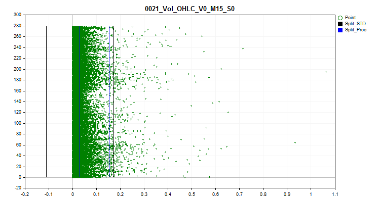
Figure 1. Determining spike definition limits

 

^2.1 This method replaces all spike values with a value close to the boundary (split). This approach makes it possible not to distort the estimate of the approximation by the quantum table within the spike boundaries.

 

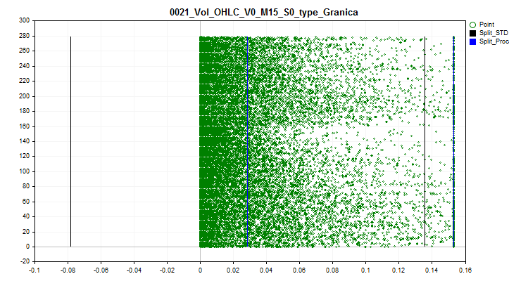
Figure 2. The spike value is converted to the value close to the split

 

^2.2 This method replaces all spike values with random values, according to the ranks within the boundaries of normal data. This approach makes it possible to dissipate the error in estimating the approximation by a quantum table.

  

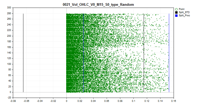
Figure 3. The spike value is converted to a random value in the range outside the spike

 

³ If it is necessary to evaluate and select quantum tables taking into account converted spikes, then select "true". When this function is activated, the array in the form of a matrix with the original data will be changed, the values of predictors with spikes will be set to the ones selected according to the spike transformation method.

⁴ You can save the train.csv sample. It will be saved to the "..\CB\Q_Vibros_Viborka" directory. This may be necessary to carry out quantization using CatBoost. Since the data will already be changed to transformed ones, the quantization tables may differ, and this may also allow reducing the number of separators (splits) to achieve a minimum error threshold when assessing the quality of approximation by a quantum table.

⁵ Activating this parameter and setting the variable to "true" will result in sequential loading of files with the train.csv, test.csv and exam.csv subsamples. In each row of the subsample, the number of predictor values in the spike region will be counted, and the total result will be recorded in the additionally created "Proc_Vibros" column. The changed selection will be saved to the "..\CB\ADD_Drop_Info_Viborka" directory.

Regardless of whether this setting is activated, a separate file will be created in the project directory at "..\CB\Proc_Vibros_Train.csv". The file contains only information about the spikes in the 'train' sample.

^5.1 Activating this setting will remove rows with spikes from the selections. Sometimes it is worth trying to train a model on data without spikes.

^5.2 If you decide to delete rows with outliers, then it is worth assessing the percentage of predictors whose value was in the spike definition area.

 

Configuring correlation estimation

• Use correlation estimation to eliminate predictors ¹
• Method for excluding correlated predictors defines the selection method (exclusion of predictors) to choose from:²
• Backward selection of predictors^2.1
• Selecting generalizing predictors^2.2
• Selecting rare predictors^2.3
• Correlation ratio³

¹ When selecting "true", the Pearson correlation estimation is activated. The result of this functionality will be to obtain a predictor correlation table at "../CB", where the file name consists of the "Corr_Matrix_" name and "Corr_Matrix_70.csv" correlation ratio size. Highly correlated predictors will be excluded.

² There are three predictor exclusion methods to choose from.

^2.1 This method searches for correlated predictors in reverse order, and if there is an earlier one, then the current column with the predictor is excluded from training.

^2.2 The method estimates the number of predictors that correlate with each predictor and iteratively selects the one that correlates with a large number of predictors eliminating other predictors that correlate with it. The logic here is that we select predictors with information that contain the most information on other predictors. Thus, we obtain data generalization.

^2.3 This method is similar to the previous one, but here we select those predictors that are least similar to others. Here there is an attempt to do the opposite - to find a predictor with unique data.

³ Here we should indicate the Pearson correlation ratio. Only after reaching or exceeding the specified ratio value are predictors considered similar for manipulation to exclude them from the sample.

 

Configuring handling time-unstable predictors

• Use testing for the mean value in each part of the sample ¹
• Subsample mean spread percentage²

¹When selecting "true", a check for fluctuations in the average value of the predictor indicator in each of the 1/10 parts of the sample is activated. This test allows excluding predictors whose indicators are highly shifted over time. Such predictors, in theory, impede training. An example of such a predictor can be seen in Figure 4, while a visual assessment can be seen in Figure 5. The example predictor was built on the basis of the Variable Index Dynamic Average (iVIDyA) indicator, which, in fact, shows the average price value, and its use in the model will lead to training behavior at a certain absolute price.

 

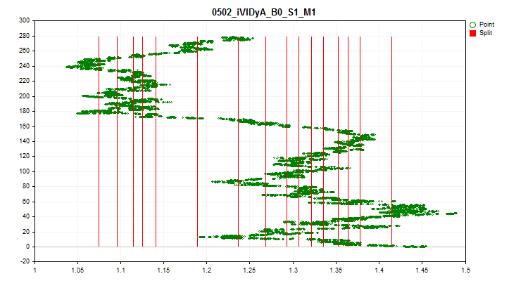
Figure 4. The iVIDyA_B0_S1_M1 predictor shows a considerable shift

  

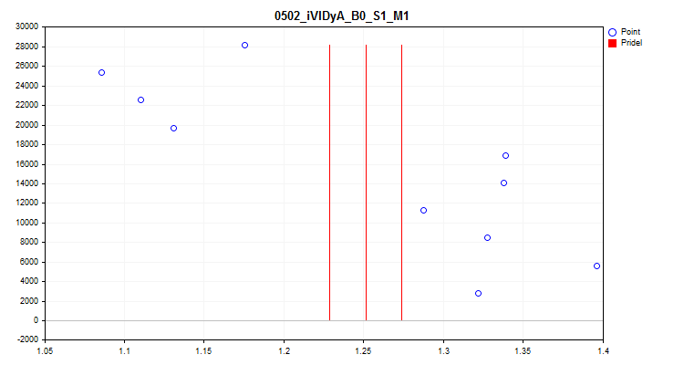
Figure 5. The iVIDyA_B0_S1_M1 predictor (mean spread)

 

² Here the width of the range is indicated as a percentage for each boundary, which is determined from the entire range of predictor values relative to the average value over the entire period.

 

Configuring the creation of a uniform quantum table

• Create a uniform quantized table¹
• The number of intervals the original data should be divided (quantized) into²

¹ When selecting "true", the algorithm for creating a uniform quantum table for all predictors in the sample is activated. The table will be saved to the Q_Bit project subdirectory.

² Set the number of intervals the predictor will be divided into.

 

Configuring the creation of a quantum table with an element of randomness

• Create a random quantum table¹
• Initial number for the random number generator ²
• Number of iterations to find the best option³
• The number of intervals the original data should be divided (quantized) into⁴

¹ When selecting "true", the algorithm for creating a random quantum table for all predictors in the sample is activated. The table will be saved to the Q_Random project.

² The number makes it possible to make the result of random generation repeatable. By changing the number, we can change the sequence of generated numbers.

³ The algorithm evaluates the approximation error after each generation of a random table and selects the best option. The more attempts, the greater the chance of finding the most successful option.

⁴ Set the number of intervals the predictor will be divided into.

 

Configuring the selection of quantum tables

• Start selecting quantum tables¹
• Use a threshold to select a predictor²
• Maximum allowed quantization error³

¹ When selecting "true", the algorithm for searching and evaluating quantum tables from the Q subdirectory of the project is activated, otherwise the program stops working. The result of executing this script function will be the creation of two directories:

The "..\CB\Setup" directory is to contain 3 files:

• Auxiliary.txt – auxiliary file with index numbers of predictors that were excluded
• Quant_CB.csv – file with quantum tables for predictors that will participate in training
• Test_CB_Setup_0_000000000 – file with information for CatBoost – columns to be excluded from training and a column to be considered as the target one.

The Test_Error directory will contain the arr_Svod.csv file. It contains the summary results of calculating the reconstruction (approximation) error for each predictor when using different quantization tables. The first column contains a list of predictors, the subsequent results when applying a specific quantum table, while the last column contains the index of the quantum table that showed the best result. The best result was used to create the Quant_CB.csv summary quantum table.

² If "false", then only the reconstruction (approximation) error is used to evaluate quantum tables, and the table that produces the smallest error is selected.

If "true", then the reconstruction (approximation) error divided by the number of splits in the quantum table is used to evaluate quantum tables. This approach allows us to take into account the number of quantum tables during estimation in order to avoid excessive quantization. The tables will only participate in the selection if their error is lower than the one specified in the next settings parameter.

³ Here we indicate the maximum acceptable error in reconstructing (approximating) predictor values.

 

Configuring saving the transformed selection

• Convert and save the sample¹
• Data conversion option:²
• Save as indices^2.1
• Save as centroids^2.2

¹ If "true", the sample (three csv files) will be converted and saved to the "..\CB\Index_Viborka" project subdirectory. This setting makes it possible to use quantum tables in those machine training algorithms where they were not originally provided. Another use case is to publicly share model training data without disclosing predictor scores to protect against the disclosure of competitive information about the data sources used. In addition, saving in the form of indices can significantly reduce the amount of disk space occupied by sample files, as well as reduce the amount of RAM for manipulating the sample.

² Select one of two options for converting predictor values after applying the final quantization summary table.

^2.1 Save the indices of the quantum table segments the predictor number falls within.

^2.2 Save the value between two boundaries the predictor number falls within.

 

Configuring graph saving

• Save the graphs¹
• Graph width²
• Graph height³
• Font size in the legend⁴

¹ If "true", the function of creating and saving graphs is activated. Graphic files containing information about each predictor in the sample will be created in the Graphics directory. The file name begins with the predictor number followed by the name of the predictor from the sample column header and the conditional graph name. Let's look at the graphs obtained for the iCCI_B0_S1_M1 predictor:

- The first graph shows the density of predictor values on a specific interval - the higher the density, the more strongly the graph curve will slope upward on this interval. The X axis is the predictor value, and the Y axis is the observation number ordered by its value. Using the graph, we can estimate the density of observations in the sample falling on specific intervals and see the spikes.

 

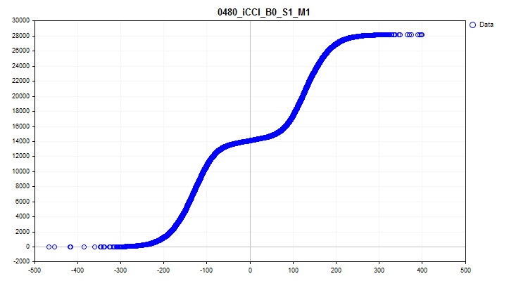
Figure 6. Density of predictor values

 

- The second graph shows at what intervals the values of the predictors were observed at the target "0" and "1". As a result, the values for zero are shown in blue, while the values for one are shown in red. Thus, it is possible to see at which predictor intervals the target value is represented to a greater extent. I recommend constructing a graph wider than the one displayed here.

 

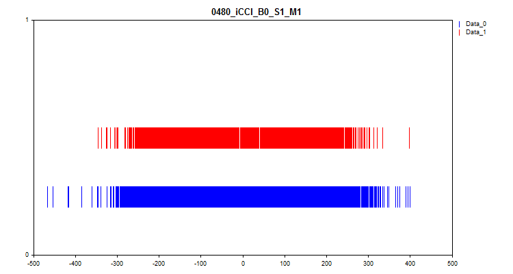
Figure 7. Correspondence of the predictor value to the target marking

 

- The third graph builds a histogram with the Y axis plotting the percentage of observations from all observations in the sample. The graph allows us to evaluate spikes and make an assumption about the distribution density.

 

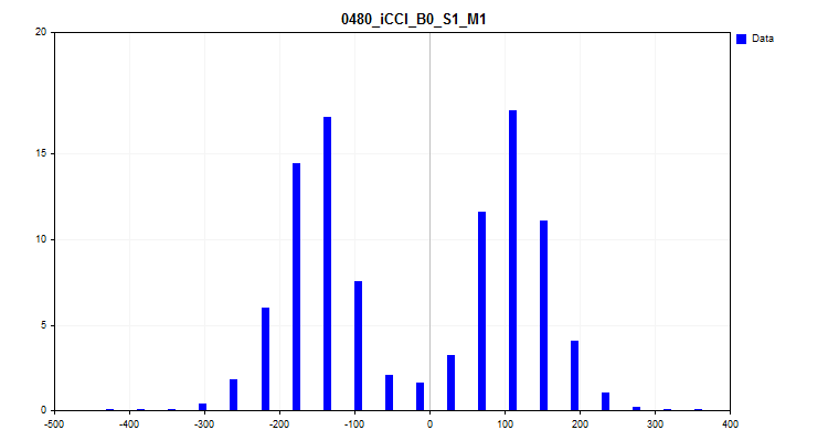
Figure 8. Distribution density histogram

 

- The fourth graph shows the filling of the predictor scale range with its values in chronological order, and also shows the levels that were selected for final quantization. The X axis is the value of the predictor, and the Y axis is the number of the group of 100 observations.

 

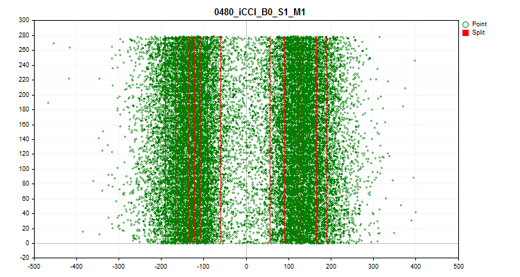
Figure 9. Quantum table

 

- The fifth graph shows the average predictor value over 10 sampling intervals. If there is a strong scatter, it is recommended to exclude the predictor. The X axis is the value of the predictor, and the Y axis is the number of the group of N observations.

 

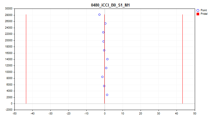
Figure 10. Average value spread

 

- The sixth graph shows the estimated spikes. There are 3 black lines on the graph - this is the average value, as well as plus and minus three standard deviations. Blue boundaries are those close to 2.5% of observations measured from the beginning and end of the sample range. The X axis is the value of the predictor, and the Y axis is the number of the group with a fixed number of observations.

 

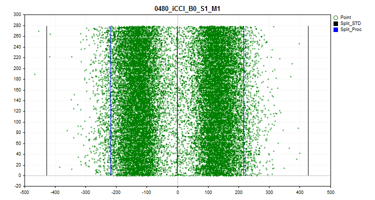
Figure 11. Spikes

 

² Graph width in pixels.

³ Graph height in pixels.

⁴ Font size and size of the curve symbols in the chart legend.

 

Configuring the search for setup scenarios

• Go through setting scenarios¹

¹ Activates the search for settings according to the embedded algorithm. Find out the details below.

2. Conducting a comparative experiment to evaluate the effect of quantization

Setting up the experiment - objectives

We have a tool with considerable functionality, it is time to evaluate its capabilities! Let's conduct an experiment that will give answers to the following pressing questions:

1. Is there any point in all these actions and manipulations with the selection of quantum tables for predictors? Maybe it would be easier to use the default CatBoost settings?
2. How many minimum splits (boundaries) are needed to achieve a similar result as with the default CatBoost settings?
3. Should we use quantization methods, such as "uniform" and "random"?
4. Is there a significant difference between quantum table selection methods?

To answer these questions, we will need to conduct training with different quantum tables obtained using different settings of the Q_Error_Selection script. I suggest trying the following settings:

Selection method:

• Only the reconstruction (approximation) error is used to evaluate quantum tables.
• the reconstruction (approximation) error divided by the number of splits in the quantum table is used to evaluate quantum tables. The maximum error is equal to 1%.
• the reconstruction (approximation) error divided by the number of splits in the quantum table is used to evaluate quantum tables. The maximum error is equal to 0.5%.

Source of quantum tables:

• Tables obtained using CatBoost.
• Tables obtained by the uniform quantization method.
• Tables obtained using the random split method.

Quantum table set:

• Set "1" - all available quantum tables in the source directory are used.
• Set "2" - only quantum tables with 16 splits or intervals are used.
• Set "3" - only quantum tables with 32 splits or intervals are used.
• Set "4" - only quantum tables with 64 splits or intervals are used.
• Set "5" - only quantum tables with 128 splits or intervals are used.
• Set "6" - only quantum tables with 256 splits or intervals are used.

  All setting combinations are displayed in the table in the form of Figure 12. In the code, this task is implemented in the form of three nested loops that change the corresponding settings activated by setting a variable in the settings called "Iterate through settings scenarios" to 'true'.

  

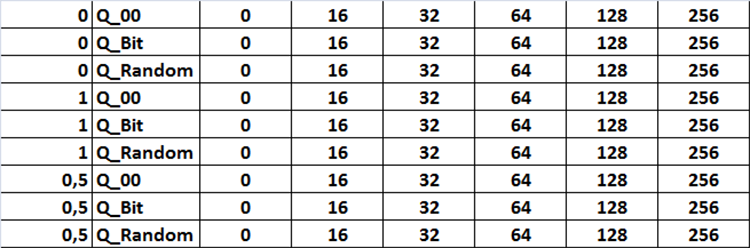
Figure 12. Table of combinations of search settings

 

 We will train 101 models with each combination of settings, moving through the Seed parameter from 0 to 800 with the step of 8, which will allow us to average the result obtained to evaluate the settings in order to exclude a random result.

These are the parameters I propose to use for comparative analysis:

• Profit_Avr - average profit of all models;
• MO_Avr - average mathematical expectation of the models;
• Precision_Avr - average classification precision of models;
• Recall_Avr - average completeness of model recalls;
• N_Exam_Model - average number of models that showed a profit of more than 3000 units;
• Profit_Max - average maximum profit of all models.

After calculating the indicators, I propose to sum them up and divide them by the number of indicators. Thus, we will obtain a general indicator of the quality of setting up the selection of quantum tables - let’s simply call it Q_Avr.

Preparing data for the experiment

To obtain a sample, we will use the same EA and scripts we used earlier when getting acquainted with CatBoost in the article "CatBoost machine learning algorithm from Yandex without learning Python or R".

I used the following settings:

A. Tester settings:

• Symbol: EURUSD
• Timeframe: M1
• Interval from 01.01.2010 to 01.09.2023

B. CB_Exp EA strategy settings:

• Period: 104
• Timeframe: 2 Minutes
• MA method: Smoothed
• Price calculation base: Close price

After receiving the sample and dividing it into 3 parts (train, test, exam), we need to obtain quantum tables in a similar way to what I described earlier in my article. To achieve this, I modified the CB_Bat script (attached to this article). Now, when selecting Brut_Quantilization_grid in the "Search object" setting, the script creates the _01_Quant_All.txt file. The settings for searching the range remained the same - the initial and final values of the variable, as well as the change step are set. I used the search from 8 to 256 with the step of 8. As a result of the script operation, commands for obtain quantization tables with all types will be prepared with a specified number of boundaries. The quantization table file will have the following naming structure: the file name in the form of the "quant" semantic file name, the number of separators and the serial number of the division type. The parameters will be linked by an underscore, the files themselves will be saved in the Q directory, which is the same as the project Setup directory.

quant_"+IntegerToString(Seed,3,'0')+"_"+IntegerToString(ENUM_feature_border_type_NAME(Q),0)+".csv"; 

After running the script, change the extension of the resulting _01_Quant_All.txt file to *.bat, place the CatBoost version previously specified in the script in the directory with the file and run the file by double-clicking on it.

When the script finishes its work, a set of files appears in the Q subdirectory - these are the quantization tables we will continue to work with.

 

 

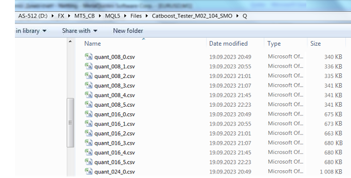
Figure 13. Q subdirectory contents

 

Using the Q_Error_Otbor script, generate uniform and random quantum tables with the number of intervals 16, 32, 64, 128 and 256. The appropriate files will appear in the Q_Bit and Q_Random directories. Make a copy of the Q directory into the project directory and name the new directory Q_00.

Now we have everything we need to create the training task package. Launch the Q_Error_Otbor script, switch the "Search settings scenarios" parameter to "true" and click "Ok". The script will create files with a quantum table and training settings according to the scenario specified in the code.

In order to use quantum tables for each configuration of CatBoost settings during training, the script adds the name of the settings file to the name of the "Quant_CB.csv" quantum table.

Let's get the files for training using the CB_Bat_v_02 script. I chose to search Seed from 0 to 800 with the step of 8 and indicated the project directory.

Now we need to slightly edit the training file replacing the file name Quant_CB.csv with Quant_CB_%%a.csv. This change will allow us to use the name of the settings as a variable, the number of which determines the number of training cycles. Copy the created files to the Setup project directory and start training by renaming the file _00_Start.txt to _00_Start.bat and double-clicking on _00_Start.bat.

 

Evaluation of the experiment results

After training is complete, we will use the CB_Calc_Svod script to calculate the metrics for each model. The script settings were previously described in detail in the previous article, so I will not repeat myself.

I also trained 101 models with the default quantum table settings. Here are the results:

•   Profit_Avr=2810.17;
•   МО_Avr=28.33;
•   Precision _Avr=0.3625;
•   Recall_Avr=0.023;
•   N_Exam_Model=43;

•   Profit_Max=8026.

  Let's take a closer look at the result tables and graphs for each parameter before drawing general conclusions.

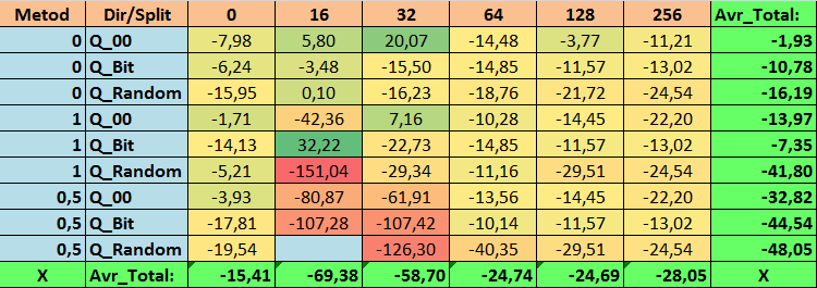
Table 14. Summary values of the Profit_Avr parameter

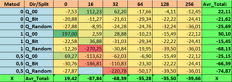
Table 15. Summary values of the MO_Avr parameter

 

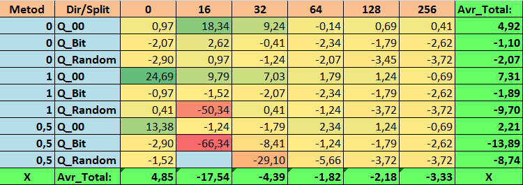
Table 16. Summary values of the Precision_Avr parameter

 

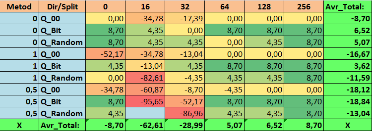
Table 17. Summary values of the Recall_Avr parameter

 

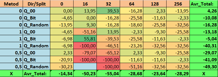
Table 18. Summary values of the N_Exam_Model parameter

 

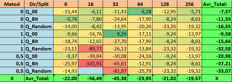
Table 19. Summary values of the Profit_Max parameter

 

Table 20. Summary values of the Q_Avr parameter

Having reviewed our informative tables, we were able to see that the spread of the parameters is quite large, which indicates the effect of the settings as a whole on the training outcome. We see that the tables obtained by randomly setting up a split (Q_Random) showed the weakest results relative to quantum tables created by other methods. It seems interesting that an increase in the number of splits generally leads to a deterioration in the performance of our metrics, with the exception of the Recall_Avr metric. This is probably due to the fact that the information in quantum segments is highly scattered, which leads to not only mathematical manipulations during training (which ends with an increase in the model confidence), but a decrease in accuracy, and then the average profit. You might ask, “how does the model train successfully with 254 splits by default?” The fact is that I use the default grid construction method called GreedyLogSum, which, as we have seen earlier, does not construct the grid with a uniform step. Due to the fact that the grid is not built uniformly, the metric we often choose to assess the quality of grid construction shows a worse result than a uniform grid. As a result, we rarely select such a method as GreedyLogSum when choosing quantization tables from the set obtained by all CatBoost methods. We can even look at statistics on how often this method was chosen. For example, in case of the (0;Q_00;256) combination, this is for only 121 predictors out of 2408. Why do the extreme parts of the predictor ranges turn out to be so significant? Write your assumptions in the comments!

The tables with a large number of splits and with the random method of setting splits did not show very good results. But what can be said about the difference in the methods for selecting quantum tables? Let's start with the bad news. The requirement for the error of 0.5% turned out to be too high for table values from 16 to 64. As a result, significantly fewer predictors participated in training than there were initially, but at the same time, tables with a large number of splits successfully overcame this threshold, but as we have already suggested, this was not efficient. However, when choosing from all available tables, the results were relatively well-balanced tables (especially the set of CatBoost tables). At the same time, the selection method for predictors having less stringent requirements (a minimum of 1% error in approximation) has shown itself to be a solution that deserves more attention.

Now let's move on to answering the questions posed - after all, answering them is the goal of this experiment.

Answers:

1. The default quantization table in CatBoost objectively shows a good result on our data, but it turns out that it can be significantly improved! Let's look at our metrics for the best methods for obtaining quantum tables:

• Profit _Avr - (1;Q_Bit;16) combination exceeding the basic settings by 32.22%.
• MO_Avr - (1;Q_00;0) combination exceeding the basic settings by 197.00%.
• Precision_Avr - (1;Q_00;0) combination exceeding the basic settings by 24.69%.
• Recall_Avr – there is a plethora of combinations here. All of them exceed the basic settings by 8.7%.
• N_Exam_Model - (1;Q_Bit;16) combination exceeding the basic settings by 55.81%.
• N_Profit_Max - (1;Q_00;32) combination exceeding the basic settings by 9.24%.

Thus, we can objectively give a positive answer to this question. It is worth trying to select the best quantum tables, which can improve the results in the metrics that are important to us.

2. It turned out that for our sample, only 16 splits are enough to get a good value for the Q_Avr parameter. For instance, in case of (1;Q_Bit;16), it is equal to 16.28, while in case of (0;Q_00;16), it is 18.24.

3. The uniform method showed itself to be quite efficient. Especially interesting is the fact that it allowed us to obtain the most models with the (1;Q_Bit;16) combination, which exceeds the basic settings by 55.81%. Given that it showed one of the best results in terms of mathematical expectation, exceeding the basic settings by 36.88%, I think it is worth using this method when choosing quantization tables and implementing it in other projects related to machine learning. As for the tables obtained by the random split method, this approach should be used with caution (perhaps selectively) where it is not possible to pass the threshold of a given criterion for selecting quantum tables. 10000 options might not be enough to find the best division of the predictor into quantum segments.

4. As the experiment results showed, the method of selecting quantum tables has a significant impact on the results. However, one experiment is not sufficient to confidently recommend using only one of the methods. Different methods and their settings allow the model to focus its attention on different parts of the data in the sample by selecting different quantum tables, which can help find the optimal solution.

 

Conclusion

In this article, we got acquainted with the algorithm for selecting quantum tables and conducted a large experiment to assess the feasibility of selecting quantum tables. Other methods of data preprocessing were superficially reviewed without analyzing the code and without assessing the efficiency of these methods. Conducting a series of experiments and describing their results is a labor-intensive task. If this article is of interest to readers, then I may conduct experiments and provide descriptions in other articles.

I did not use balance charts in the article. Although there are some nice examples of models, but I would recommend using more predictors to select and subsequently build models for real trading in financial markets.

The approximation score was used to select quantum tables, but it is worth trying other scores that can assess the homogeneity and usefulness of the data.

#	Application	Description
1	Q_Error_Otbor.mq5	Script responsible for data preprocessing and selection of quantum tables for each predictor.
2	CB_Bat_v_02.mq5	Script responsible for generating tasks for training models using CatBoost - new version 2.0
3	CSV fast.mqh	Class for working with CSV files, all copyrights to the program code belong to Aliaksandr Hryshyn. You need to download the missing files here.