
Neural networks made easy (Part 14): Data clustering
Contents
- Introduction
- 1. Unsupervised learning
- 2. The k-means algorithm
- 3. Python Implementation
- 4. Testing
- Conclusion
- List of references
- Programs used in the article
Introduction
In this series of articles, we have already made a substantial progress in studying various neural network algorithms. But all previously considered algorithms were based on supervised model learning principles. It means that we input some historical data into the model and optimized weights so that the model returned values very close to reference results. In practice, this approach usually generates maximum results. But to implement this learning process, in addition to the historical data for the training sample, we also need reference results for each state of the system. As you understand, the preparation of reference values involves additional labor costs when preparing a training sample. Furthermore, it is not always possible to give an unambiguous reference result for each system state. As a consequence, this imposes restrictions on the possible size of the training sample.
There is another approach to Artificial Intelligence learning methods — unsupervised learning. This method enables model training only using the original data, without the need to provide reference values. This reduces labor costs when preparing the training sample. This in turn enables the use of more input data to train the model. However, the ragne of possible tasks will also be limited.
In this article, you will not see the previously used vertical structure of a neural network consisting of several neural layers. But first things first. Let's consider the possible algorithms and see how they can be used in trading.
1. Unsupervised learning
Usually, three separate areas are distinguished in the AI algorithm development field:
- Supervised learning
- Unsupervised learning
- Reinforcement learning
As can be understood from the names, their main difference is in the approaches to training the models. The first method, Supervised Learning, was considered in detail in previous articles within this series. To implement this method, we need a training set with pairs of labeled values "system state - correct output". In practice, this approach usually generates maximum results. However, it also requires additional resources (including human resources) and time to prepare a labeled training set. Furthermore, it is not always possible to find an unambiguous reference result for each system state. At the same time, we must take into account the human factor with a certain degree of probability. Sometimes, these reasons serve as the major restrictions in generating a training dataset.
So, what can we do when there is a lot of initial data but little knowledge about them? Or when it is not possible to label a certain reference value for each state of the learning process? Or when we even do not know what this reference value should be? These are quite frequent cases during the initial acquaintance with a large amount of data. Instead of spending resources on finding correct reference output for each system state, we will switch to unsupervised learning. Depending on the task, the unsupervised model learning can be used either to get a solution to the problem or to pre-process the initial data.
Please note that the problems solved by supervised and unsupervised learning methods are very different. For example, it is impossible to solve regression problems using unsupervised learning. One might compare classification tasks solved by the supervised learning method and clustering problems solved by unsupervised learning algorithms. However, behind the similar meaning of these two words there is a completely different logic. Often these two methods generate completely different results. When using supervised classification, we offer the model to learn which of the system states corresponds to which class. With unsupervised clustering, we offer the model to independently determine which cluster to attribute the state of the system to, based on a set of features describing this state. In this case, we may not even know the number of such clusters at the beginning of work. This number is a hyperparameter of the system, which can be selected in the process of model training.
The second problem solved with through unsupervised learning algorithms is the search for anomalies. It means that the model should search for the states which are not characteristic of a given system, but which can appear with a small degree of probability due to various external factors.
Another problem solved by unsupervised learning algorithms is data dimensionality reduction. Remember, previous article we solved a similar problem using convolutional networks. However, in supervised learning, we were looking for specific features which are characteristic of this specific task. In contrast, in unsupervised learning we have to compress data with minimal information lost.
If we take a look at all the problems solved by unsupervised learning algorithms, we can say that the main task of such an approach is to study and generalize features found in input data. With this approach, the model can independently study the features describing the system state. This is also often used in solving supervised learning problems. In this case, a model is first trained using unsupervised learning algorithms on a large amount of data. The system should learn the features of the system as well as possible. As the next step, the model is trained to solve a specific problem using a small amount of labeled data.
As you can see, unsupervised learning algorithms can be used to solve various problems. But how can they be used in trading? Let's think. Graphical analysis methods almost always involve certain chart patterns: Double Top / Double Bottom, Head and Shoulders, Flag, various harmonic patterns, etc. Furthermore, there are a lot of smaller patterns consisting of 1-3 candlesticks. But when we try to describe a particular pattern in mathematical language, have to deal with a large number of conventions and tolerances. This complicates their use in algorithmic trading. Even when a human trader determines the patterns, there is a lot of subjectivity. That is why, when analyzing the same chart, different traders find identify patterns on it, which often have opposite directed predictive movements. Well, perhaps this is the underlying rule of trading as a whole. Some make profit, others lose. In the trading process, no new commodity-material values are created, while the money supply remains unchanged. It only moves from one wallet to another. So, how can we avoid loss?
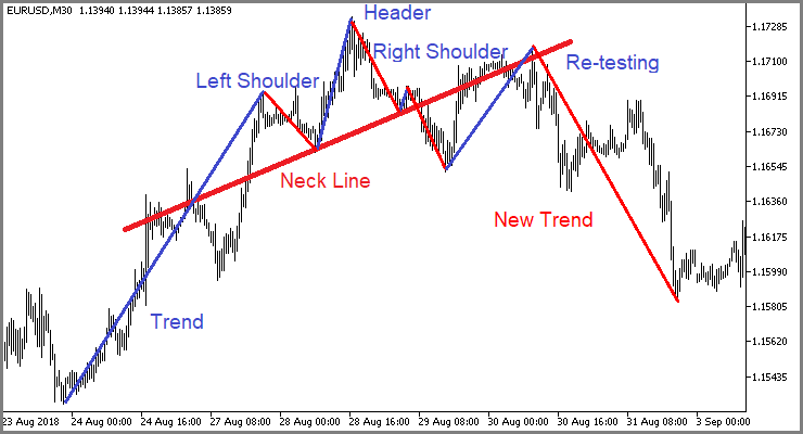
Let's once again take a look at the chart patterns mentioned above. Yes, they all have their variations. But at the same time, each pattern has its own specific structure, which identifies it against the general price movement chart. So, what if we use unsupervised data clustering algorithms to let the model identify all possible variations in the data over a certain time period. Since we use unsupervised learning, there is no need to label the data, as well as the time period can be quite large. However, do not forget that an increase in the history time period increases model training costs.
2. The k-means algorithm
To solve the clustering problem proposed above, we will use one of the simplest and most understandable methods: k-means. Despite its simplicity, the method is effective in solving data clustering problems and can be used either on its own or for data preprocessing.
To enable the method use, each state of the system must be described by a certain set of data collected into a single vector. Each such vector represents the coordinates of a point in the N-dimensional space. The space dimension is equal to the dimension of the system state description vector.
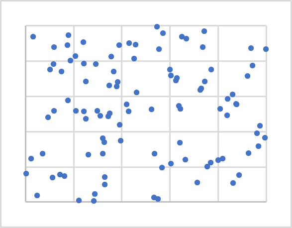
The idea of the method is to find such centers (vectors) around which all known states of the system can be combined into clusters. The average distance of all states of the system to the center of the corresponding cluster should be minimal. This is where the method name k-means comes from. The number of such clusters is a hyperparameter of the model. It is determined at the model design or validation stage.
The phrase "... determined at the model design or validation stage" may sound a little strange. These concepts seem to be separated in time and by stages of model creation and training. But the cases are different. Sometimes, the number of such clusters is specified when setting the problem. This happens is the customer clearly understands the number of clusters based on prior experience or on the planned use. Or the number of distinct clusters can be clearly seen during data visualization. In such cases, we can immediately indicate to the model the number of clusters we are looking for.
In other cases, when we do not have sufficient knowledge to unambiguously determine the number of clusters, we will have to conduct a model training series in order to determine the optimal number of clusters. We will get back to it a little later. Now let's analyze the method operation algorithm.
The figure above shows the visualization of random 100 points on a plane. Data visualization assists in understanding its structure but is however not required for this method. As you can see, the points are distributed quite evenly over the entire plane, and we cannot visually clearly distinguish any clusters. And thus, we cannot know their number. For the first experiment, we will use, for example, 5 clusters.
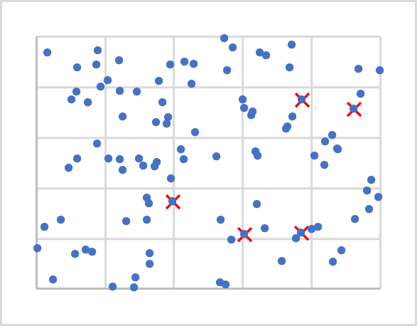
Now that we know the number, where should we locate their centers? Do you remember, that when we initialized weights, we filled the matrices with random values? We will do roughly the same here. But we will not generate random vectors as they can be left out of our initial data. We will simply take 5 random points from our training set. They are marked by X in the figure below.
Next, we need to calculate the distance from each point to each center. I guess that finding the distance between two points on a line (1-dimensional space) is not that difficult. To determine the distance between two points on a plane, we will use the Pythagorean theorem which we know from the school mathematics. The theorem states that the sum of the squares of the legs is equal to the square of the hypotenuse. Therefore, the distance between two points on the plane is equal to the square root of the sum of the squared distances between the projections of the points on the coordinate axes. Simply put, it is the sum of the squares of the difference of the corresponding coordinates. If we apply a similar approach for the projection of a point onto an N-1 plane, we will obtain a similar equality for an N-dimensional space.

We know the distance to each of the cluster centers, and the nearest of them will determine that the point belongs to this cluster. Repeat the iterations to determine the distances and the cluster for all points of our training sample. After that, determine a new center for each cluster using a simple arithmetic mean. The figure below shows the results of the first iteration. The points of each cluster are colored in a separate color.
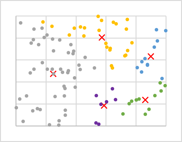
As you can see, after the first iteration, points are distributed across clusters unevenly. But cluster centers have been shifted in comparison with the previous chart. And therefore, during repeated recalculations of the distances to cluster centers, during which we also determine whether a point belongs to this or that cluster, the distribution of points over clusters will change.
We repeat such iterations until the cluster centers stop moving. Also, the clusters to which points belong will no longer be changed.
After several iterations for our data sample, we have the following result. As you can see, we have a fairly uniform distribution of training sequence points over clusters.
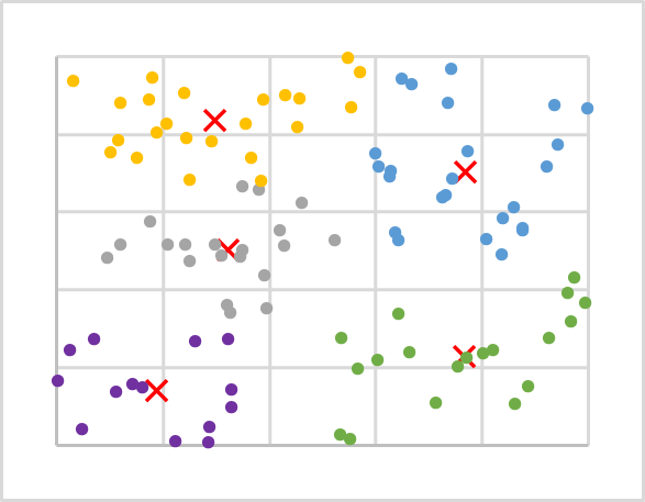
Let's summarize the considered algorithm:
- Determine k random points from the training sample as cluster centers.
- Organize a cycle of operations:
- Determine the distance from each point to each center
- Find the nearest center and assign a point to this cluster
- Using the arithmetic mean, determine a new center for each cluster.
- Repeat the operations in a loop until cluster centers "stop moving".
In this example, we are not interested in the specific distance from a point to the center, while we only need to find the shortest one. Therefore, to save resources, we will not calculate the square root of the resulting sum when calculating the distance, as this will absolutely not affect the data clustering result.
At this stage, we have divided our training sample data into clusters. Next, how do we determine that this number of clusters is optimal? As with the supervised learning, we introduce a loss function that will help us evaluate the quality of the trained model as well as compare the performance of the model when using different hyperparameters. For clustering problems, such a loss function is the average deviation of points from the corresponding cluster center. It is calculated by the following formula:
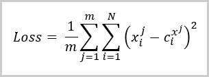
Where:
- m is the number of elements in the training sample
- N is the size of the description vector of one element form the training sample
- Xi jis the i-th value of the description vector of the j-th element from the training sample
- Ci x jis the i-th value of the central vector of the class to which the j-th element from the training sample belongs.
It can be seen from the above formula, the value of the loss function will be equal to 0 when the number of clusters is equal to the number of elements in the training sample. But we do not want to copy the entire training sample into our matrix of cluster centers. On the contrary, we want to find a way to generalize the data so that we can then look for possible patterns for each cluster.
I repeated the clustering of the same training set with a different number of clusters. The figure below shows the dependence of the loss function on the number of clusters. I did not show the loss function values, since they can be very different for different input data. At the same time, the number of clusters also depends on the training sample, and thus you should not rely on the given values. They are provided here only to explain the graph. It is important to understand chart interpretation principles.
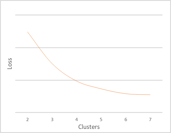
The above graph clearly shows that when the number of clusters changes from 2 to 4, the value of the error function decreases sharply. As the number of clusters further increases to 6, the rate of decrease in the error function value gradually decreases. When the number of clusters changes from 6 to 7, the value of the error function practically does not change. This is a smoothed change in the loss function. But sometimes there can be a broken graph change at a specific point. This phenomenon often occurs when the training data is clearly separable.
The general rule for interpreting the graph is as follows:
- When a graph has a broken line, the optimal number of clusters is at the break point.
- When the graph is smoothed, find the balance between the quality and performance in the bend zone.
Given the small sample sizes and the number of clusters, I would recommend using 5 or 6 clusters for our example.
3. Python Implementation
We have discussed the theoretical aspects of the k-means method using abstract data as an example. And the reasonable question is, how does the method work on real data? To answer this question, we will use the integration of MetaTrader 5 and Python. Python offers a large number of libraries which can cover almost any need.
The integration tools have already been mentioned many times on this site, while the library installation procedure is described in the documentation.
3.1. Include libraries
To implement the task, we will use several libraries. First, the MetaTrader5 library. This library implements all points of MetaTrader 5 terminal integration with Python.
The second library we will use is Scikit-Learn. This library offers simple and effective tools for data analysis. In particular, it implements several data clustering algorithms. One of them is the k-means method we are considering.
Data visualization will be implemented using the Matplotlib library.
Using MetaTrader 5 and Python integration tools, information about the account status, trading operations and market situation can be transferred to scripts. However, they do not allow the use of data of internal program, such as indicators. Therefore, we will need to reproduce the entire implementation of the indicators on the Python side. To make the task easier, we will use the TA-Lib library which offers different technical analysis tools.
Before proceeding to creating the script, install all these libraries and Python interpreter on your computer. This process is beyond the scope of this article. However, if you have any difficulties, I will answer in the comments to the article.
3.2. Creating a script
Now that we have decided on the list of libraries to use, we can start writing the script. Save the script code as "clustering.py".
At the beginning of the script, include the necessary libraries.
# Import Libraries
import numpy as np
import matplotlib.pyplot as plt
import MetaTrader5 as mt5
from talib import abstract as tl
import sklearn.cluster as cluster
from datetime import datetime as dt
Next, organize connection to the terminal. Check the operation correctness. In case of an error, display a relevant message and exit the program.
# Connect to the MetaTrader 5 terminal
if not mt5.initialize():
    print("initialize() failed, error code =",mt5.last_error())
    quit()
Upon successful connection to the terminal, download historical data for the analyzed period and disconnect from the terminal.
# Downloading quotes
rates=mt5.copy_rates_range('EURUSD',mt5.TIMEFRAME_H1,dt(2006,1,1),dt(2022,1,1))
mt5.shutdown()
Now that the historical data is available, let's move on to determining indicator values. In this block, we will calculate the values of the same indicators that we used when testing various models with supervised learning. These are classical oscillators: RSI, CCI and MACD.
# Calculate indicator values
rsi=tl.RSI(rates['close'])
cci=tl.CCI(rates['high'],rates['low'],rates['close'])
macd,macdsignal,macdhist=tl.MACD(rates['close'])
Now we have source data, but it is split into 6 tensors. They need to be combined into one tensor for analysis. Please pay attention to the following. The clustering function is constructed in such a way that it receives a 2-dimensional array as input; the lines of this array are considered as separate patterns. By combining all the tensors into one, we also get a 2-dimensional array, each line of which contains information about one individual candlestick. It could be used in this form. But this would be clustering of individual candlesticks. Will this information be useful? If we want to look for patterns consisting of several candlesticks, then we need to change the dimension of the tensor. But a simple change in dimension does not quite satisfy our requirements. This is like using a rolling window with a move step equal to its size. But we need to know the pattern at each candlestick. Therefore, we will need to reformat the tensor with data copying. The example below shows code for combining a tensor and then copying the data to create a pattern of 20 candlesticks. Note the cutoff of historical data, where the indicator values are not defined.
# Group the training sample
data=np.array([rates['close']-rates['open'],rates['high']-rates['close'],rates['close']-rates['low'],
                                                                   rsi,cci,macd,macdsignal,macdhist]).T
s=data.shape[0]
data=np.hstack([data[40+k:s-20+k] for k in range(0,20)])
This completes the data preparation process. Now we can proceed to data clustering. But in order to estimate the required number of clusters, we need to conduct several tests with a different number of clusters. In this example, I performed clustering for a range of 50 to 1000 clusters, in increments of 50 clusters.
# Perform clustering with a different number of clusters
R=range(50,1000,50)
KM = (cluster.KMeans(n_clusters=k).fit(data) for k in R)
Then determine the error for each case and visualize the data obtained.
distance=(k.transform(data) for k in KM)
dist = (np.min(D, axis=1) for D in distance)
avgWithinSS = [sum(d) / data.shape[0] for d in dist]
# Plotting the model training results
plt.plot(R, avgWithinSS)
plt.xlabel('$Clasters$')
plt.title('Loss dynamic')
# Display generated graphs
plt.show()
This concludes the work with the script code. Coming next is testing. The full code of the script is attached to the article.
4. Testing
We have created a Python script and can test it. All testing parameters are specified in the script code:
- Symbol EURUSD
- Timeframe H1
- Historical interval: 16 years from 01/01/2006 to 01/01/2022
- Number of clusters: from 50 to 1000 in increments of 50
Below is the graph showing the dependence of the loss function on the number of clusters.
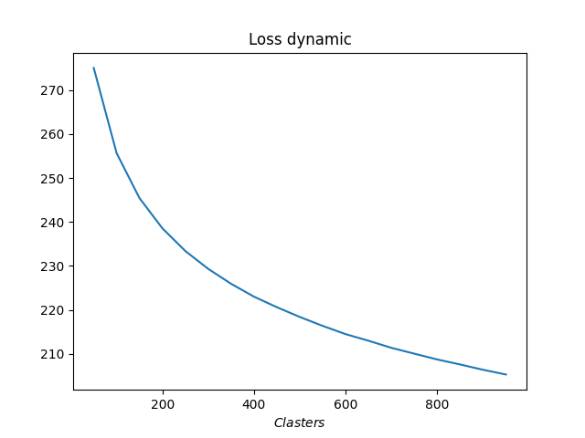
As you can see on the graph, the transition turned out to be quite stretched. The optimal number of clusters appeared to be from 400 to 500. Totally we have analyzed 98,641 states of the system.
Conclusion
This article introduces the reader to the k-means data clustering method, which is one of the unsupervised learning algorithms. We have created a script using Python libraries and trained the model with a different number of clusters. Based on testing results, we can conclude that the model was able to identify about 500 patterns. Of course, not all of them will give clear signals for trading operations. We will talk about how to use the results obtained in practice in the following articles.
List of references
- Neural networks made easy
- Neural networks made easy (Part 2): Network training and testing
- Neural networks made easy (Part 3): Convolutional networks
- Neural networks made easy (Part 4): Recurrent networks
- Neural networks made easy (Part 5): Multithreaded calculations in OpenCL
- Neural networks made easy (Part 6): Experimenting with the neural network learning rate
- Neural networks made easy (Part 7): Adaptive optimization methods
- Neural networks made easy (Part 8): Attention mechanisms
- Neural networks made easy (Part 9): Documenting the work
- Neural networks made easy (Part 10): Multi-Head Attention
- Neural networks made easy (Part 11): A take on GPT
- Neural networks made easy (Part 12): Dropout
- Neural networks made easy (Part 13): Batch Normalization
Programs used in the article
| # | Name | Type | Description |
|---|---|---|---|
| 1 | clustering.py | Script | Data Clustering - Python Script |
Translated from Russian by MetaQuotes Ltd.
Original article: https://www.mql5.com/ru/articles/10785
Warning: All rights to these materials are reserved by MetaQuotes Ltd. Copying or reprinting of these materials in whole or in part is prohibited.
This article was written by a user of the site and reflects their personal views. MetaQuotes Ltd is not responsible for the accuracy of the information presented, nor for any consequences resulting from the use of the solutions, strategies or recommendations described.
 MQL5 Wizard techniques you should know (Part 02): Kohonen Maps
 Indicators with on-chart interactive controls
 Developing a trading Expert Advisor from scratch (Part 14): Adding Volume At Price (II)
 Learn how to design a trading system by Williams PR
- Free trading apps
- Over 8,000 signals for copying
- Economic news for exploring financial markets
You agree to website policy and terms of use
Hi Dmitriy
I install all libraries but when i try to run this python rogram i get this error:
runfile('C:/Users/rogerio/ título1.py', wdir='C:/Users/rogerio')
Traceback (most recent call last):
File "C:\Users\rogerio\sem título1.py", line 20, in <module>
rsi=tl.RSI(rates['close'])
TypeError: 'NoneType' object is not subscriptable
I am using this source code
# -------------------------------------------------------#
# Data clustering model #
# -------------------------------------------------------#
# Import Libraries
import numpy as np
import matplotlib.pyplot as plt
import MetaTrader5 as mt5
from talib import abstract as tl
import sklearn.cluster as cluster
from datetime import datetime as dt
# Connect to the MetaTrader 5 terminal
if not mt5.initialize():
print("initialize() failed, error code =",mt5.last_error())
quit()
# Downloading quotes
rates=mt5.copy_rates_range('EURUSD',mt5.TIMEFRAME_H1,dt(2006,1,1),dt(2022,1,1))
mt5.shutdown()
# Calculate indicator values
rsi=tl.RSI(rates['close'])
cci=tl.CCI(rates['high'],rates['low'],rates['close'])
macd,macdsignal,macdhist=tl.MACD(rates['close'])
# Group the training sample
data=np.array([rates['close']-rates['open'],rates['high']-rates['close'],rates['close']-rates['low'],rsi,cci,macd,macdsignal,macdhist]).T
s=data.shape[0]
data=np.hstack([data[40+k:s-20+k] for k in range(0,20)])
# Perform clustering with a different number of clusters
R=range(50,1000,50)
KM = (cluster.KMeans(n_clusters=k).fit(data) for k in R)
distance=(k.transform(data) for k in KM)
dist = (np.min(D, axis=1) for D in distance)
avgWithinSS = [sum(d) / data.shape[0] for d in dist]
# Plotting the model training results
plt.plot(R, avgWithinSS)
plt.xlabel('$Clasters$')
plt.title('Loss dynamic')
# Display generated graphs
plt.show()
Thans for help
Rogerio
Hello Rogerio.
Do you have install TA-Lib : Technical Analysis Library?