
Neural Networks in Trading: Point Cloud Analysis (PointNet)

Introduction
Point clouds are simple and unified structures that avoid combinatorial inconsistencies and complexities associated with meshes. Since point clouds do not have a conventional format, most researchers typically convert such datasets into regular 3D voxel grids or image sets before passing them into a deep network architecture. However, this conversion makes the resulting data unnecessarily large and can introduce quantization artifacts, often obscuring the natural invariances of the data.
For this reason, some researchers have turned to an alternative representation of 3D geometry, using point clouds directly. Models operating with such raw data representations must account for the fact that a point cloud is merely a set of points and is invariant to permutations of its elements. This necessitates a certain degree of symmetrization in the model's computations.
One such solution is described in the paper "PointNet: Deep Learning on Point Sets for 3D Classification and Segmentation". The model introduced in this work, named PointNet, is a unified architectural solution that directly takes a point cloud as input and outputs either class labels for the entire dataset or segmentation labels for individual points within the dataset.
The basic architecture of the model is remarkably simple. At the initial stages, each point is processed identically and independently. In the default configuration, each point is represented solely by its three coordinates (x, y, z). Additional dimensions can be incorporated by computing normals and other local or global features.
The key aspect of the PointNet approach is the use of a single symmetric function MaxPooling. Essentially, the network learns a set of optimization functions that select significant or informative elements within the point cloud and encode the reasoning behind their selection. The fully connected layers at the output stage aggregate these learned optimal values into a global descriptor for the entire shape.
This input data format is easily compatible with rigid or affine transformations since each point is transformed independently. Consequently, the authors of the method introduce a data-dependent spatial transformation model, which attempts to canonicalize the data before processing it in PointNet, further enhancing the efficiency of the solution.
1. The PointNet Algorithm
The authors of PointNet developed a deep learning framework that directly utilizes unordered point sets as input data. A point cloud is represented as a set of 3Dpoints {Pi|i=1,…,n}, where each point Pi is a vector of its coordinates (x, y, z) plus additional feature channels, such as color and other attributes.
The model’s input data represents a subset of points from Euclidean space, characterized by three key properties:
- Unordered. Unlike pixel arrays in images, a point cloud is a set of elements without a defined order. In other words, a model consuming a set of N 3D points must be invariant to the N! permutations of the input dataset order.
- Point interactions. The points exist in a space with a distance metric. This means they are not isolated; rather, neighboring points form meaningful subsets. Consequently, the model must be capable of capturing local structures from nearby points as well as combinatorial interactions between local structures.
- Transformation invariance. As a geometric entity, the learned representation of a point set should be invariant to specific transformations. For instance, simultaneous rotation and translation of the points should not alter the global category of the point cloud or its segmentation.
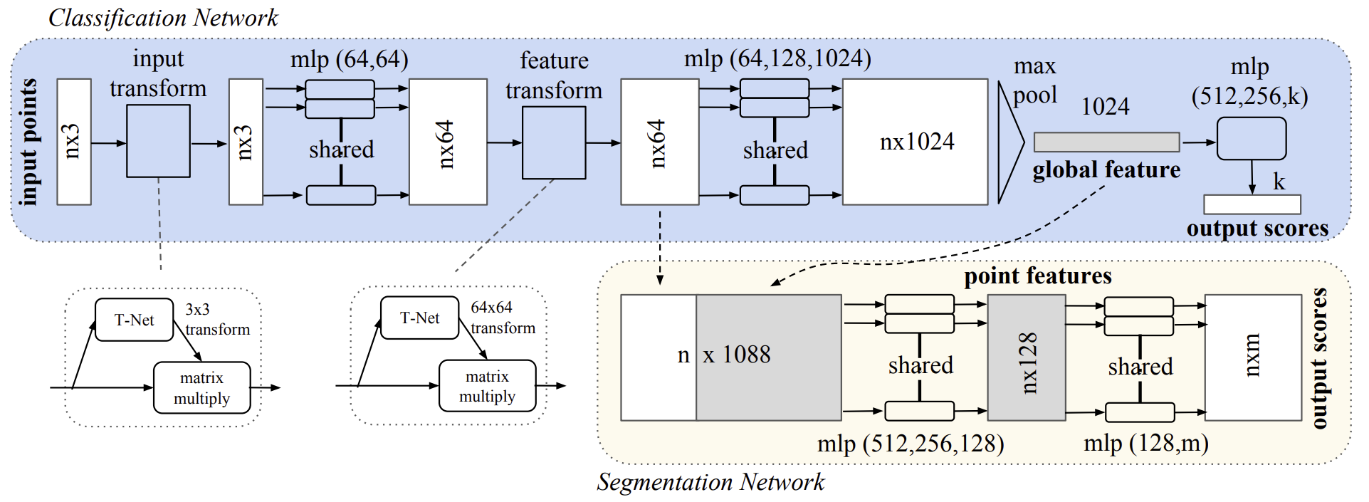
The PointNet architecture is designed so that classification and segmentation models share a large portion of their structure. It consists of three key modules:
- A max-pooling layer as a symmetric function for aggregating information from all points.
- A structure for combining local and global data representations.
- Two joint alignment networks that align both the raw input points and the learned feature representations.
To ensure the model is invariant to the permutation of input data, three strategies are proposed:
- Sorting the input data into a canonical order.
- Treating the input data as a sequence for training an RNN, but supplementing the training set with all possible permutations.
- Using a simple symmetric function to aggregate information from each point. A symmetric function takes n vectors as input and outputs a new vector that is invariant to the order of the input.
Sorting the source data sounds like a simple solution. However, in a multidimensional space, there is no ordering that would be stable under point perturbations in the general sense. Therefore, sorting does not solve the ordering problem completely. This makes it difficult for the model to learn a consistent mapping between input and output data. Experimental results have shown that applying MLP directly to a sorted set of points performs poorly, though slightly better than processing raw unsorted data.
While RNNs demonstrate reasonable robustness to input order for short sequences (tens of elements), scaling them to thousands of input elements is challenging. Empirical results presented in the original paper also show that an RNN-based model does not outperform the proposed PointNet algorithm.
The core idea of PointNet is to approximate a general function defined over a set of points by applying a symmetric function to transformed elements within the set:
![]()
Empirically, the authors propose a basic module that is highly simple: first, h is approximated using an MLP, and g is composed of a single-variable function and a max-pooling function. Experimental validation confirms the effectiveness of this approach. Through a collection of h functions, a range of f functions can be learned to capture various properties of the input dataset.
Despite the simplicity of this key module, it exhibits remarkable properties and achieves high performance across multiple applications.
At the output of the proposed key module, a vector [f1,…,fK] is formed, serving as the global signature of the input dataset. This enables the training of an SVM or MLP classifier on the global feature shape for classification tasks. However, point-wise segmentation requires a combination of local and global knowledge. This can be achieved in a simple yet highly effective manner.
After computing the global feature vector for the entire point cloud, the authors of PointNet propose feeding this vector back to each individual point object by concatenating the global representation with each point. This allows new per-point features to be extracted based on the combined point-wise objects - now considering both local and global information.
With this modification, PointNet can predict per-point scores based on both local geometry and global semantics. For example, it can accurately predict normals for each point, demonstrating that the model is able to summarize information from the local neighborhood of the point. Experimental results from the original study show that the proposed model achieves state-of-the-art performance in shape part segmentation and scene segmentation tasks.
Semantic labeling of point clouds should remain invariant when the point cloud undergoes certain geometric transformations, such as rigid transformations. Therefore, the authors expect the learned point-set representation to be invariant to such transformations.
A natural solution is to align the entire input set to a canonical space before feature extraction. The point cloud input format allows us to achieve this goal in a simple way. We just need to predict an affine transformation matrix using a mini-network (T-net) and directly apply this transformation to the input point coordinates. The mini-network itself resembles the larger network and consists of basic modules for point-independent feature extraction, max-pooling, and fully connected layers.
This idea can be extended to feature space alignment. An additional alignment network can be inserted at the point feature level to predict a feature transformation matrix for aligning objects from different input point clouds. However, the feature-space transformation matrix has a much higher dimensionality than the spatial transformation matrix, significantly increasing optimization complexity. Therefore, the authors introduce a regularization term in the SoftMax loss function. For this, we constrain the feature transformation matrix to be close to an orthogonal matrix:
![]()
where A is the feature alignment matrix predicted by the mini-network.
Orthogonal transformations do not result in information loss at the input stage, making them desirable. The authors of PointNet found that adding this regularization term stabilizes optimization and improves model performance.
Author's visualization of the PointNet method is presented below.
2. Implementation in MQL5
In the previous section, we explored the theoretical foundation of the approaches proposed in PointNet. Now, it is time to move on to the practical part of this article, where we will implement our own version of the proposed approaches using MQL5.
2.1 Creating the PointNet Class
To implement PointNet algorithms in code, we will create a new class, CNeuronPointNetOCL, inheriting the base functionality from the fully connected layer CNeuronBaseOCL. The structure of the new class is shown below.
class CNeuronPointNetOCL   :  public CNeuronBaseOCL
  {
protected:
   CNeuronPointNetOCL   *cTNet1;
   CNeuronBaseOCL       *cTurned1;
   CNeuronConvOCL       cPreNet[2];
   CNeuronBatchNormOCL  cPreNetNorm[2];
   CNeuronPointNetOCL   *cTNet2;
   CNeuronBaseOCL       *cTurned2;
   CNeuronConvOCL       cFeatureNet[3];
   CNeuronBatchNormOCL  cFeatureNetNorm[3];
   CNeuronTransposeOCL  cTranspose;
   CNeuronProofOCL      cMaxPool;
   CNeuronBaseOCL       cFinalMLP[2];
   //---
   virtual bool         OrthoganalLoss(CNeuronBaseOCL *NeuronOCL, bool add = false);
   //---
   virtual bool      feedForward(CNeuronBaseOCL *NeuronOCL) override ;
   //---
   virtual bool      calcInputGradients(CNeuronBaseOCL *NeuronOCL) override;
   virtual bool      updateInputWeights(CNeuronBaseOCL *NeuronOCL) override;

public:
                     CNeuronPointNetOCL(void) {};
                    ~CNeuronPointNetOCL(void);
   //---
   virtual bool      Init(uint numOutputs, uint myIndex, COpenCLMy *open_cl,
                          uint window, uint units_count, uint output, bool use_tnets,
                          ENUM_OPTIMIZATION optimization_type, uint batch);
   //---
   virtual int       Type(void) override   const   {  return defNeuronPointNetOCL; }
   //---
   virtual bool      Save(int const file_handle) override;
   virtual bool      Load(int const file_handle) override;
   //---
   virtual bool      WeightsUpdate(CNeuronBaseOCL *source, float tau) override;
   virtual void      SetOpenCL(COpenCLMy *obj) override;
  };
You should be already used to observing a large number of nested objects in the class structure. However, this case has its own nuances. First, alongside static objects, we also have several dynamic ones. In the class destructor, we must remove them from the device's memory.
CNeuronPointNetOCL::~CNeuronPointNetOCL(void)
  {
   if(!!cTNet1)
      delete cTNet1;
   if(!!cTNet2)
      delete cTNet2;
   if(!!cTurned1)
      delete cTurned1;
   if(!!cTurned2)
      delete cTurned2;
  }
However, we do not create these objects in the class constructor, allowing us to keep it empty.
The second nuance is that two of the nested dynamic objects are instances of the class we are creating, CNeuronPointNetOCL. So, they are nested inside nested objects.
Both of these nuances stem from the authors' approach to aligning input data and features to a certain canonical space. We will discuss this further during the implementation of our class methods.
The initialization of a new instance of the class object, as usual, is implemented in the Init method. The parameters of this method include key constants defining the architecture of the created object.
In this case, the algorithm is designed for point cloud classification. The general idea is to build an Environmental State Encoder using PointNet approaches. This encoder returns a probability distribution mapping the current environmental state to a particular type. The Actor's policy then maps a specific environmental state type to a set of trade parameters that potentially yield maximum profitability in the given state. From this, the main parameters of the class architecture emerge:
- window — size of the parameter window for a single point in the analyzed cloud;
- units_count — number of points in the cloud;
- output — size of the result tensor;
- use_tnets — whether to create models for projecting input data and features into canonical space.
The output parameter specifies the total size of the result buffer. It should not be confused with the previously used result window parameter. In this case, we expect the output to be a descriptor of the analyzed environmental state. The result tensor size logically corresponds to the number of possible environmental state classification types.
bool CNeuronPointNetOCL::Init(uint numOutputs, uint myIndex, COpenCLMy *open_cl,
                              uint window, uint units_count, uint output, bool use_tnets,
                              ENUM_OPTIMIZATION optimization_type, uint batch)
  {
   if(!CNeuronBaseOCL::Init(numOutputs, myIndex, open_cl, output, optimization_type, batch))
      return false;
In the body of the method, as usual, we first invoke the identically named method of the parent class, which already implements the minimum necessary validation of the received parameters and the initialization of inherited objects. At the same time, we ensure that we check the execution results of the method operations.
Next, we proceed with the initialization of nested objects. Initially, we verify whether it is necessary to create internal models for projecting the source data and features into canonical space.
//--- Init T-Nets
   if(use_tnets)
     {
      if(!cTNet1)
        {
         cTNet1 = new CNeuronPointNetOCL();
         if(!cTNet1)
            return false;
        }
      if(!cTNet1.Init(0, 0, OpenCL, window, units_count, window * window, false, optimization, iBatch))
         return false;
If projection models need to be created, we first check the validity of the pointer to the model object and, if required, instantiate a new object of the CNeuronPointNetOCL class. Following this, we proceed with its initialization.
Note that the size of the source data for the projection matrix generation object matches the size of the source data received by the main class from the external program. However, the result buffer size equals the square of the source data window. This is because the output of this model is expected to be a square matrix for projecting the source data into canonical space. Furthermore, we explicitly set the parameter indicating the necessity of creating projection matrices for the source data and features to false. This prevents uncontrolled recursive object creation. Additionally, embedding transformation models for source data within another transformation model for source data would be illogical.
Finally, we verify the pointer to the object responsible for recording the corrected data and, if necessary, create a new instance of the object.
      if(!cTurned1)
        {
         cTurned1 = new CNeuronBaseOCL();
         if(!cTurned1)
            return false;
        }
      if(!cTurned1.Init(0, 1, OpenCL, window * units_count, optimization, iBatch))
         return false;
And we initialize this inner layer. Its size corresponds to the tensor of the original data.
We perform similar operations for the feature projection model. The only difference is in the dimensions of the inner layers.
      if(!cTNet2)
        {
         cTNet2 = new CNeuronPointNetOCL();
         if(!cTNet2)
            return false;
        }
      if(!cTNet2.Init(0, 2, OpenCL, 64, units_count, 64 * 64, false, optimization, iBatch))
         return false;
      if(!cTurned2)
        {
         cTurned2 = new CNeuronBaseOCL();
         if(!cTurned2)
            return false;
        }
      if(!cTurned2.Init(0, 3, OpenCL, 64 * units_count, optimization, iBatch))
         return false;
     }
Next we form an MLP of the primary extraction of point features. At this stage, the authors of PointNet propose an independent extraction of point features. Therefore, we replace fully connected layers with convolutional layers having a step size equal to the size of the window of the analyzed data. In our case, they are equal to the size of the vector describing one point.
//--- Init PreNet
   if(!cPreNet[0].Init(0, 0, OpenCL, window, window, 64, units_count, optimization, iBatch))
      return false;
   cPreNet[0].SetActivationFunction(None);
   if(!cPreNetNorm[0].Init(0, 1, OpenCL, 64 * units_count, iBatch, optimization))
      return false;
   cPreNetNorm[0].SetActivationFunction(LReLU);
   if(!cPreNet[1].Init(0, 2, OpenCL, 64, 64, 64, units_count, optimization, iBatch))
      return false;
   cPreNet[1].SetActivationFunction(None);
   if(!cPreNetNorm[1].Init(0, 3, OpenCL, 64 * units_count, iBatch, optimization))
      return false;
   cPreNetNorm[1].SetActivationFunction(None);
Between the convolutional layers, we insert batch normalization layers and apply the activation function to them. In this case, we use 2 layers of each type with the dimensions proposed by the authors of the method.
Similarly, we add a three-layer perceptron for higher-order feature extraction.
//--- Init Feature Net
   if(!cFeatureNet[0].Init(0, 4, OpenCL, 64, 64, 64, units_count, optimization, iBatch))
      return false;
   cFeatureNet[0].SetActivationFunction(None);
   if(!cFeatureNetNorm[0].Init(0, 5, OpenCL, 64 * units_count, iBatch, optimization))
      return false;
   cFeatureNet[0].SetActivationFunction(LReLU);
   if(!cFeatureNet[1].Init(0, 6, OpenCL, 64, 64, 128, units_count, optimization, iBatch))
      return false;
   cFeatureNet[1].SetActivationFunction(None);
   if(!cFeatureNetNorm[1].Init(0, 7, OpenCL, 128 * units_count, iBatch, optimization))
      return false;
   cFeatureNetNorm[1].SetActivationFunction(LReLU);
   if(!cFeatureNet[2].Init(0, 8, OpenCL, 128, 128, 512, units_count, optimization, iBatch))
      return false;
   cFeatureNet[2].SetActivationFunction(None);
   if(!cFeatureNetNorm[2].Init(0, 9, OpenCL, 512 * units_count, iBatch, optimization))
      return false;
   cFeatureNetNorm[2].SetActivationFunction(None);
Essentially, the architecture of the last two blocks is identical. They differ only in the number of layers and their sizes. Logically, they could be combined into a single block. However, in this case, they are separated solely to allow for the insertion of a feature transformation block into canonical space between them.
The next stage, following the extraction of point features, involves applying the MaxPooling function as specified by the PointNet algorithm. This function selects the maximum value for each feature vector element from the entire analyzed point cloud. As a result, the point cloud is represented by a feature vector containing the maximum values of the corresponding elements from all points in the analyzed cloud.
We already have the CNeuronProofOCL class in our toolkit, which performs a similar function but in a different dimension. Therefore, we first transpose the obtained point feature matrix.
   if(!cTranspose.Init(0, 10, OpenCL, units_count, 512, optimization, iBatch))
      return false;
And then we form a vector of maximum values.
   if(!cMaxPool.Init(512, 11, OpenCL, units_count, units_count, 512, optimization, iBatch))
      return false;
The obtained descriptor of the analyzed point cloud is processed by a three-layer MLP. However, in this case, I decided to resort to a little trick and declared only 2 internal fully connected layers. For the third layer, we use the created object itself, since it inherited all the necessary functionality from the parent class.
//--- Init Final MLP
   if(!cFinalMLP[0].Init(256, 12, OpenCL, 512, optimization, iBatch))
      return false;
   cFinalMLP[0].SetActivationFunction(LReLU);
   if(!cFinalMLP[1].Init(output, 13, OpenCL, 256, optimization, iBatch))
      return false;
   cFinalMLP[1].SetActivationFunction(LReLU);
At the end of the class object initialization method, we explicitly specify the activation function and return the logical result of the operations to the calling program.
   SetActivationFunction(None);
//---
   return true;
  }
After completing the implementation of the initialization method of our new class, we move on to constructing the feed-forward pass algorithms for PointNet. This is done in the feedForward method. As before, in the parameters of this method, we receive a pointer to the source data object.
bool CNeuronPointNetOCL::feedForward(CNeuronBaseOCL *NeuronOCL)
  {
//--- PreNet
   if(!cTNet1)
     {
      if(!cPreNet[0].FeedForward(NeuronOCL))
         return false;
     }
In the body of the method, we immediately see a branching of the algorithm, depending on the need to project the original data into the canonical space. Please note that when initializing the object, we saved in the internal variables a flag indicating the need to perform data projection. However, to check whether a data projection is necessary, we can use the validation of pointers to the corresponding objects. This is because projection models are created only when necessary. They are absent by default.
Therefore, if there is no valid pointer to the model object for generating the projection matrix of the original data, we simply pass the obtained pointer to the original data object to the feed-forward method of the first convolutional layer of the pre-feature extraction block.
If it is necessary to project data into canonical space, we pass the received data to the feed-forward pass method of the model to generate the data transformation matrix.
   else
     {
      if(!cTurned1)
         return false;
      if(!cTNet1.FeedForward(NeuronOCL))
         return false;
At the output of the projection model, we obtain a square data transformation matrix. Accordingly, we can determine the dimension of the data window by the size of the result tensor.
int window = (int)MathSqrt(cTNet1.Neurons());
We then use matrix multiplication to obtain a projection of the original point cloud into canonical space.
      if(IsStopped() ||
         !MatMul(NeuronOCL.getOutput(), cTNet1.getOutput(), cTurned1.getOutput(), NeuronOCL.Neurons() / window,
                                                                                                window, window))
         return false;
The projection of the initial points in the canonical space is then input into the first layer of the primary feature extraction block.
      if(!cPreNet[0].FeedForward(cTurned1.AsObject()))
         return false;
     }
At this stage, regardless of the need to project the original data into the canonical space, we have already performed a feed-forward pass of the first layer of the primary feature extraction block. Then we sequentially call the feed-forward pass methods of all layers of the specified block.
   if(!cPreNetNorm[0].FeedForward(cPreNet[0].AsObject()))
      return false;
   if(!cPreNet[1].FeedForward(cPreNetNorm[0].AsObject()))
      return false;
   if(!cPreNetNorm[1].FeedForward(cPreNet[1].AsObject()))
      return false;
Next, we are faced with the question of the need to project the features of points into a canonical space. Here the algorithm is similar to the projection of the initial points.
//--- Feature Net
   if(!cTNet2)
     {
      if(!cFeatureNet[0].FeedForward(cPreNetNorm[1].AsObject()))
         return false;
     }
   else
     {
      if(!cTurned2)
         return false;
      if(!cTNet2.FeedForward(cPreNetNorm[1].AsObject()))
         return false;
      int window = (int)MathSqrt(cTNet2.Neurons());
      if(IsStopped() ||
         !MatMul(cPreNetNorm[1].getOutput(), cTNet2.getOutput(), cTurned2.getOutput(),
                                     cPreNetNorm[1].Neurons() / window, window, window))
         return false;
      if(!cFeatureNet[0].FeedForward(cTurned2.AsObject()))
         return false;
     }
After that. we complete the operations of extracting features of points of the analyzed cloud of initial data.
   if(!cFeatureNetNorm[0].FeedForward(cFeatureNet[0].AsObject()))
      return false;
   uint total = cFeatureNet.Size();
   for(uint i = 1; i < total; i++)
     {
      if(!cFeatureNet[i].FeedForward(cFeatureNetNorm[i - 1].AsObject()))
         return false;
      if(!cFeatureNetNorm[i].FeedForward(cFeatureNet[i].AsObject()))
         return false;
     }
In the next step, we transpose the resulting feature tensor. Then we form a descriptor vector for the analyzed cloud.
   if(!cTranspose.FeedForward(cFeatureNetNorm[total - 1].AsObject()))
      return false;
   if(!cMaxPool.FeedForward(cTranspose.AsObject()))
      return false;
Next, according to the PointNet classification algorithm, we need to processing of the received data in MLP. Here we perform feed-forward pass operations on the 2 internal fully connected layers.
   if(!cFinalMLP[0].FeedForward(cMaxPool.AsObject()))
      return false;
   if(!cFinalMLP[1].FeedForward(cFinalMLP[0].AsObject()))
      return false;
Then we call a similar method of the parent class, passing a pointer to the inner layer.
   if(!CNeuronBaseOCL::feedForward(cFinalMLP[1].AsObject()))
      return false;
//---
   return true;
  }
Let me remind you that in this case, the parent class is a fully connected layer. Accordingly, when calling the feed-forward pass method of the parent class, we are executing the feed-forward pass of the fully connected layer. The only difference is that, this time, we use objects inherited from the parent class rather than those of a nested layer.
Once all operations of our feed-forward pass method have been successfully completed, we return a Boolean value indicating the executed operations to the calling program.
At this point, we conclude our work on the feed-forward method and move on to the backpropagation pass methods, which are divided into two parts: error gradient distribution and model parameter adjustment.
As we have mentioned multiple times, error gradient distribution follows the exact same algorithm as the feed-forward pass, except that the flow of information is reversed. However, in this case, there is a specific nuance. For data projection matrices, the authors of the PointNet method introduced a regularization technique that ensures the projection matrix is as close as possible to an orthogonal matrix. These regularization operations do not affect the feed-forward pass algorithm; they are only involved in optimizing the model parameters. Moreover, performing these operations will require additional computations within the OpenCL program.
To begin, let's examine the proposed regularization formula.
![]()
It is evident that the authors leverage the property that multiplying an orthogonal matrix by its transposed copy results in an identity matrix.
If we break it down, multiplying a matrix by its transposed copy means that each element in the resulting matrix represents the dot product of two corresponding rows. For an orthogonal matrix, the dot product of a row with itself should produce 1. In all other cases, the dot product of two different rows yields 0.
However, it is important to note that we are dealing with regularization within the backpropagation pass. This means that we not only need to compute the error but also calculate the error gradient for each element.
To implement this algorithm within the OpenCL program, we will create a kernel named OrthogonalLoss. The parameters of this kernel will include pointers to two data buffers. One of them contains the original matrix and the other is used for storing the corresponding error gradients. Additionally, we will introduce a flag to specify whether the gradient values should be overwritten or accumulated with previously stored values.
__kernel void OrthoganalLoss(__global const float *data,
                             __global float *grad,
                             const int add
                            )
  {
   const size_t r = get_global_id(0);
   const size_t c = get_local_id(1);
   const size_t cols = get_local_size(1);
In this case, we do not indicate the dimensions of the matrices. But here everything is quite simple. We plan to run the kernel in a two-dimensional task space according to the number of rows and columns in the matrix.
In the kernel body, we immediately identify the current thread in both dimensions of the task space.
It is also worth remembering that we are dealing with a square matrix. Therefore, to understand the full size of the matrix, we only need to determine the number of threads in one of the dimensions.
To distribute vector multiplication operations across multiple threads, we create local workgroups within the rows of the original matrix. And to organize the process of data exchange between threads, we will use an array in the local memory of the OpenCL context.
   __local float Temp[LOCAL_ARRAY_SIZE];
   uint ls = min((uint)cols, (uint)LOCAL_ARRAY_SIZE);
Next we define offset constants to the required objects in the source data buffer.
   const int shift1 = r * cols + c;
   const int shift2 = c * cols + r;
We load the values of the corresponding elements from the data buffer.
   float value1 = data[shift1];
   float value2 = (shift1==shift2 ? value1 : data[shift2]);
Note that to minimize global memory accesses, we avoid re-reading diagonal elements.
Here we immediately check the validity of the obtained values, replacing invalid numbers with zero values.
   if(isinf(value1) || isnan(value1))
      value1 = 0;
   if(isinf(value2) || isnan(value2))
      value2 = 0;
After that, we calculate their product with the mandatory check of the result for validity.
   float v2 = value1 * value2;
   if(isinf(v2) || isnan(v2))
      v2 = 0;
The next step is to organize a loop of parallel summation of the obtained values in individual elements of the local array with mandatory synchronization of the workgroup threads.
   for(int i = 0; i < cols; i += ls)
     {
      //---
      if(i <= c && (i + ls) > c)
         Temp[c - i] = (i == 0 ? 0 : Temp[c - i]) + v2;
      barrier(CLK_LOCAL_MEM_FENCE);
     }
Then we create a loop to sum the obtained values of the elements of the local array.
   uint count = min(ls, (uint)cols);
   do
     {
      count = (count + 1) / 2;
      if(c < ls)
         Temp[c] += (c < count && (c + count) < cols ? Temp[c + count] : 0);
      if(c + count < ls)
         Temp[c + count] = 0;
      barrier(CLK_LOCAL_MEM_FENCE);
     }
   while(count > 1);
We also pay special attention to synchronizing workgroup threads.
As a result of the operations performed in the first element of the local array, we obtain the value of the product of the two analyzed rows of the matrix. Now we can calculate the error value.
   const float sum = Temp[0];
   float loss = -pow((float)(r == c) - sum, 2.0f);
However, this is only part of the job. Next, we need to determine the error gradient for each element of the original matrix. First, we calculate the error gradient at the level of the vector product.
float g = (2 * (sum - (float)(r == c))) * loss;
Then we propagate the error gradient to the first element in the product of the current thread values.
g = value2 * g;
Make sure to check the validity of the value of the obtained error gradient.
   if(isinf(g) || isnan(g))
      g = 0;
After that, we save it in the corresponding element of the global error gradient buffer.
   if(add == 1)
      grad[shift1] += g;
   else
      grad[shift1] = g;
  }
Here, we must check the flag that determines whether the error gradient value should be added to or overwritten, and we execute the corresponding operation accordingly.
It is important to note that within the kernel, we compute the error gradient for only one of the elements in the product. The gradient for the second element in the product will be calculated in a separate thread, where the row and column indices of the matrix are swapped.
This kernel is placed in the execution queue with the CNeuronPointNetOCL::OrthogonalLoss method. Its algorithm fully adheres to the fundamental principles of placing OpenCL program kernels into execution queues, which have been extensively covered in previous articles. I encourage you to independently review the code for this method. It is provided in the attached file.
Now, let's take a closer look at the algorithm behind the error gradient distribution method calcInputGradients. As before, this method takes as a parameter a pointer to the previous layer's object, which in this case acts as the recipient of the error gradient at the raw data level.
bool CNeuronPointNetOCL::calcInputGradients(CNeuronBaseOCL *NeuronOCL)
  {
   if(!NeuronOCL)
      return false;
In the body of the method, we immediately check the relevance of the received pointer. Otherwise, there is no point in further operations.
We then pass the error gradient through the point cloud descriptor interpretation perceptron.
   if(!CNeuronBaseOCL::calcInputGradients(cFinalMLP[1].AsObject()))
      return false;
   if(!cFinalMLP[0].calcHiddenGradients(cFinalMLP[1].AsObject()))
      return false;
We propagate the error gradient through the MaxPooling layer and transpose it into the features of the corresponding points.
   if(!cMaxPool.calcHiddenGradients(cFinalMLP[0].AsObject()))
      return false;
   if(!cTranspose.calcHiddenGradients(cMaxPool.AsObject()))
      return false;
Then we propagate the error gradient through the feature extraction layers of the points, of course in reverse order.
   uint total = cFeatureNet.Size();
   for(uint i = total - 1; i > 0; i--)
     {
      if(!cFeatureNet[i].calcHiddenGradients(cFeatureNetNorm[i].AsObject()))
         return false;
      if(!cFeatureNetNorm[i - 1].calcHiddenGradients(cFeatureNet[i].AsObject()))
         return false;
     }
   if(!cFeatureNet[0].calcHiddenGradients(cFeatureNetNorm[0].AsObject()))
      return false;
Up to this point, everything is pretty normal. But we have come to the level of point feature projection into the canonical space. Of course, if this is not required, we simply pass the error gradient to the primary feature extraction block.
   if(!cTNet2)
     {
      if(!cPreNetNorm[1].calcHiddenGradients(cFeatureNet[0].AsObject()))
         return false;
     }
If we do need to implement this, the algorithm will be more complex. First, we propagate the error gradient down to the data projection level.
   else
     {
      if(!cTurned2)
         return false;
      if(!cTurned2.calcHiddenGradients(cFeatureNet[0].AsObject()))
         return false;
After this, we distribute the error gradient between the point features and the projection matrix. If we look a few steps ahead, we can see that the error gradient will also be propagated to the point feature level through the projection matrix generation model. To prevent overwriting critical data later, we will not pass the error gradient to the final layer of the preliminary feature extraction block at this stage, but instead to the penultimate layer.
As a reminder, the last layer in the preliminary feature extraction block is the batch normalization layer. The layer before it is a convolutional layer responsible for independent feature extraction from individual points. Both layers have identically sized error gradient buffers, allowing us to substitute buffers safely without the risk of exceeding buffer boundaries.
      int window = (int)MathSqrt(cTNet2.Neurons());
      if(IsStopped() ||
         !MatMulGrad(cPreNetNorm[1].getOutput(), cPreNet[1].getGradient(), cTNet2.getOutput(),
                     cTNet2.getGradient(), cTurned2.getGradient(), cPreNetNorm[1].Neurons() / window,
                                                                                       window, window))
         return false;
After splitting the error gradient across the two data threads, we add the regularization error gradient at the projection matrix level.
      if(!OrthoganalLoss(cTNet2.AsObject(), true))
         return false;
Next, we propagate the error gradient through the projection matrix generation block.
      if(!cPreNetNorm[1].calcHiddenGradients((CObject*)cTNet2))
         return false;
And we sum the error gradient from two information threads.
      if(!SumAndNormilize(cPreNetNorm[1].getGradient(), cPreNet[1].getGradient(), cPreNetNorm[1].getGradient(),
                                                                                         1, false, 0, 0, 0, 1))
         return false;
     }
And then we can propagate the error gradient through the primary feature extraction block to the level of the original data projection.
   if(!cPreNet[1].calcHiddenGradients(cPreNetNorm[1].AsObject()))
      return false;
   if(!cPreNetNorm[0].calcHiddenGradients(cPreNet[1].AsObject()))
      return false;
   if(!cPreNet[0].calcHiddenGradients(cPreNetNorm[0].AsObject()))
      return false;
Here we apply an algorithm similar to the error gradient distribution via feature projection. The simplest version of the algorithm is the one without a data projection matrix. We simply pass the error gradient into the previous layer's buffer.
   if(!cTNet1)
     {
      if(!NeuronOCL.calcHiddenGradients(cPreNet[0].AsObject()))
         return false;
     }
But if we need to project data, we first propagate the error gradient to the projection level.
      if(!cTurned1)
         return false;
      if(!cTurned1.calcHiddenGradients(cPreNet[0].AsObject()))
         return false;
And then we distribute the error gradient across two threads depending on their influence on the result.
      int window = (int)MathSqrt(cTNet1.Neurons());
      if(IsStopped() ||
         !MatMulGrad(NeuronOCL.getOutput(), NeuronOCL.getGradient(), cTNet1.getOutput(), cTNet1.getGradient(),
                     cTurned1.getGradient(), NeuronOCL.Neurons() / window, window, window))
         return false;
We add the regularization value to the resulting error gradient.
      if(!OrthoganalLoss(cTNet1, true))
         return false;
Here, we encounter a problem with overwriting the error gradient. At this stage, we do not have free buffers available for storing data. When distributing the error gradient in two directions, we immediately wrote it into the buffer of the preceding layer. Now, we need to propagate the error gradient through the projection matrix generation block, whose operations will overwrite the gradient values, leading to the loss of previously stored data. To prevent data loss, we need to copy the gradient values to a suitable data buffer. But where can we find such a buffer? When initializing the class, we did not create buffers for storing intermediate data. However, upon closer inspection, we notice the data projection recording layer. Its size is identical to the size of the original data tensor. Additionally, the error gradient stored in this layer has already been distributed across two computation paths and will not be used in subsequent operations.
At the same time, the equality of buffer sizes suggests an alternative approach. Instead of copying the data directly, what if we swap the buffer pointers? Pointer swapping is significantly cheaper than a full data copy and is independent of the buffer size.
      CBufferFloat *temp = NeuronOCL.getGradient();
      NeuronOCL.SetGradient(cTurned1.getGradient(), false);
      cTurned1.SetGradient(temp, false);
After rearranging the pointers to the data buffers, we can pass the error gradient from the data projection matrix to the level of the previous layer.
      if(!NeuronOCL.calcHiddenGradients(cTNet1.AsObject()))
         return false;
      if(!SumAndNormilize(NeuronOCL.getGradient(), cTurned1.getGradient(), NeuronOCL.getGradient(),
                                                                            1, false, 0, 0, 0, 1))
         return false;
     }
//---
   return true;
  }
At the end of the method operations, we sum the error gradient from the two information threads and return the logical result of the method operations to the calling program.
The update of trainable model parameters is handled by the updateInputWeights method. As usual, its algorithm is simple: we sequentially invoke identically named methods of internal objects containing trainable parameters. At the same time, we ensure to call the corresponding method of the parent class, as its functionality is used as the third layer in the MLP-based point cloud descriptor evaluation. In this article, we will not go into detail about the implementation of this method. I encourage you to review its code independently in the attached files.
This concludes our consideration of the algorithms for constructing CNeuronPointNetOCL class methods. In the attachment to this article you will find the complete code of this class and all its methods.
2.2 Model architecture
After implementing the PointNet-based approaches using MQL5, we now proceed to integrate a new object into the architecture of our models. As mentioned earlier, our new class CNeuronPointNetOCL is incorporated into the Environment State Encoder model, which is defined in the CreateEncoderDescriptions method.
It is important to highlight that we have implemented nearly the entire algorithm within a single block. This enables us to construct a model with a concise and compact high-level architecture. I emphasize the term "high-level architecture" here. Despite the simple naming of the CNeuronPointNetOCL block, it encapsulates a highly complex and multi-layered neural network architecture.
As usual, the input to the model consists of raw, unprocessed data, which is normalized using a batch normalization layer to ensure compatibility.
bool CreateEncoderDescriptions(CArrayObj *&encoder)
  {
//---
   CLayerDescription *descr;
//---
   if(!encoder)
     {
      encoder = new CArrayObj();
      if(!encoder)
         return false;
     }
//--- Encoder
   encoder.Clear();
//--- Input layer
   if(!(descr = new CLayerDescription()))
      return false;
   descr.type = defNeuronBaseOCL;
   int prev_count = descr.count = (HistoryBars * BarDescr);
   descr.activation = None;
   descr.optimization = ADAM;
   if(!encoder.Add(descr))
     {
      delete descr;
      return false;
     }
//--- layer 1
   if(!(descr = new CLayerDescription()))
      return false;
   descr.type = defNeuronBatchNormOCL;
   descr.count = prev_count;
   descr.batch = 1e4;
   descr.activation = None;
   descr.optimization = ADAM;
   if(!encoder.Add(descr))
     {
      delete descr;
      return false;
     }
After that we immediately pass them to our new PointNet block.
//--- layer 2
   if(!(descr = new CLayerDescription()))
      return false;
   descr.type = defNeuronPointNetOCL;
   descr.window = BarDescr;                        // Variables
   descr.count = HistoryBars;                      // Units
   descr.window_out = LatentCount;                 // Output Dimension
   descr.step = int(true);                         // Use input and feature transformation
   descr.batch = 1e4;
   descr.activation = None;
   descr.optimization = ADAM;
   if(!encoder.Add(descr))
     {
      delete descr;
      return false;
     }
It is worth noting here that we have not specified the activation function at the output of our CNeuronPointNetOCL block. This step is taken intentionally to provide the user with the ability to extend the architecture of the point cloud identification block. However, in this experiment, we will only add a SoftMax layer to translate the obtained results into the domain of probabilistic values.
//--- layer 3
   if(!(descr = new CLayerDescription()))
      return false;
   descr.type = defNeuronSoftMaxOCL;
   descr.count = LatentCount;
   descr.activation = None;
   descr.optimization = ADAM;
   descr.layers = 1;
   if(!encoder.Add(descr))
     {
      delete descr;
      return false;
     }
//---
   return true;
  }
This completes the architecture of our new Environmental State Encoder model.
It should be said that we also simplified the architecture of the Actor and Critic models. In them, we replaced the multi-headed cross-attention block with a simple data concatenation layer. But I suggest you familiarize yourself with these specific edits in the attachment.
A few words should be said about model training programs. The change in the model architecture did not affect the structure of the source data and results, which allows us to use previously created programs for interaction with the environment and the data they collected for offline training. However, the dataset we collected earlier lacks class labels for the selected environmental states. Creating them would require additional costs. We decided to take a different path and train the Environmental State Encoder in the process of Actor policy training. Therefore, we excluded the individual Environmental State Encoder training EA "StudyEncoder.mq5". Instead, we have made minor edits to the Actor and Critic training EA "Study.mq5" to enable it to train the Environmental State Encoder. I suggest you familiarize with them independently.
Let me remind you that in the attachment, you will find the full code of the class presented in this article and all its methods, as well as the algorithms of all the programs used in preparing the article. We now move on to the final stage of our work - testing and evaluating the results of the work done.
3. Testing
In this article, we introduced the new PointNet method for processing raw data in the form of point clouds and realized our vision of the authors' proposed approaches using MQL5. Now, it is time to assess the effectiveness of the proposed approaches in solving our tasks. To do so, we will train the models discussed in the article using real historical data from the EURUSD instrument. For our experiment, we will use historical data from 2023 as the training dataset. The models will then be tested using January 2024 data. In both cases, we will use the H1 timeframe and default parameters for all analyzed indicators.
In essence, we have used unchanged training and testing parameters for the models across several articles. Therefore, the initial training is conducted using previously collected datasets.
At the same time, the training of the Environment State Encoder occurs simultaneously with the Actor policy training. As you know, the Actor policy is trained iteratively, with periodic updates to the training dataset. This approach ensures that the training dataset remains relevant and aligned with the current Actor policy's action space. This in turn allows for a more fine-tuned training process.
After several iterations of training the models, we managed to obtain an actor policy that generates profits on both the training and test datasets. The test results are presented below.
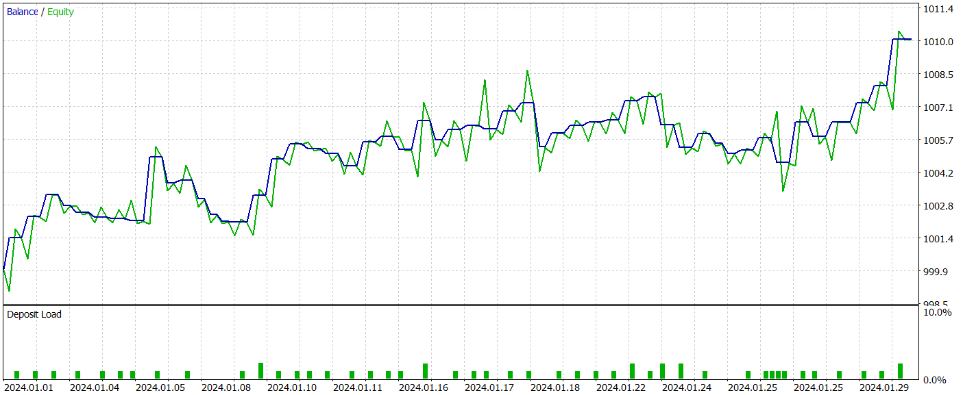
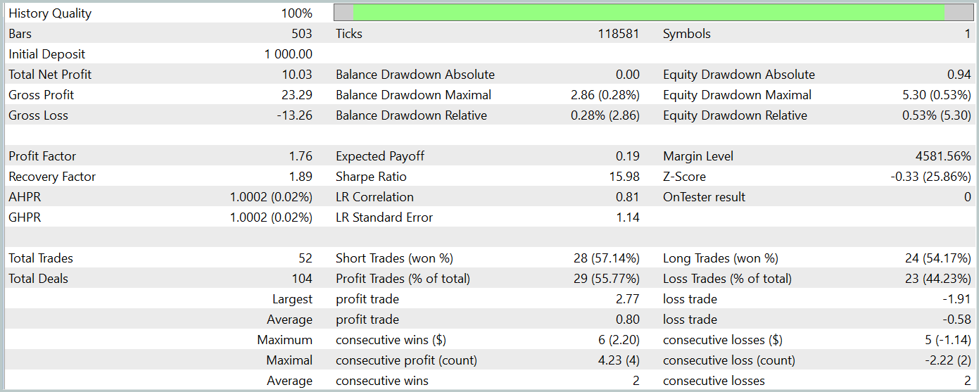
During the testing period, the model executed 52 trades, with 55.77% of them closing profitably. It is worth noting that the model exhibits a practical parity between long and short positions (24 vs. 28, respectively). Both the maximum and average profitable trades exceeded the corresponding loss positions. The profit factor reached 1.76. The balance curve shows a clear upward trend. However, the short testing period and the relatively low number of trades do not allow us to conclude the stability of the learned policy over an extended period.
In summary, the implemented approaches are promising but require further testing.
Conclusion
In this article, we got acquainted with a new method PointNet, which is a unified architectural solution that directly takes the point cloud as input data. The application of PointNet in trading enables the effective analysis of complex multidimensional data, such as price patterns, without the need to convert them into other formats. This opens up new opportunities for more accurate forecasting of market trends and improvement of decision-making algorithms. Such analysis can potentially improve the efficiency of trading strategies in financial markets.
In the practical part of the article, we implemented our vision of the proposed approaches in MQL5, trained models on real historical data and tested the Expert Advisor using the learned policy in the MetaTrader 5 strategy tester. Based on the testing results, we obtained promising results. However, it should be remembered that all programs presented in this article are provided for informational purposes only and are created only to demonstrate the capabilities of the proposed approaches. Significant refinement and comprehensive testing in all possible conditions, as well as thorough testing are required before real life use.
Programs used in the article
| # | Issued to | Type | Description |
|---|---|---|---|
| 1 | Research.mq5 | Expert Advisor | EA for collecting examples |
| 2 | ResearchRealORL.mq5 | Expert Advisor | EA for collecting examples using the Real-ORL method |
| 3 | Study.mq5 | Expert Advisor | Model training EA |
| 4 | Test.mq5 | Expert Advisor | Model testing EA |
| 5 | Trajectory.mqh | Class library | System state description structure |
| 6 | NeuroNet.mqh | Class library | A library of classes for creating a neural network |
| 7 | NeuroNet.cl | Library | OpenCL program code library |
Translated from Russian by MetaQuotes Ltd.
Original article: https://www.mql5.com/ru/articles/15747
Warning: All rights to these materials are reserved by MetaQuotes Ltd. Copying or reprinting of these materials in whole or in part is prohibited.
This article was written by a user of the site and reflects their personal views. MetaQuotes Ltd is not responsible for the accuracy of the information presented, nor for any consequences resulting from the use of the solutions, strategies or recommendations described.


- Free trading apps
- Over 8,000 signals for copying
- Economic news for exploring financial markets
You agree to website policy and terms of use