
Neural Networks in Trading: Hierarchical Vector Transformer (Final Part)

Introduction
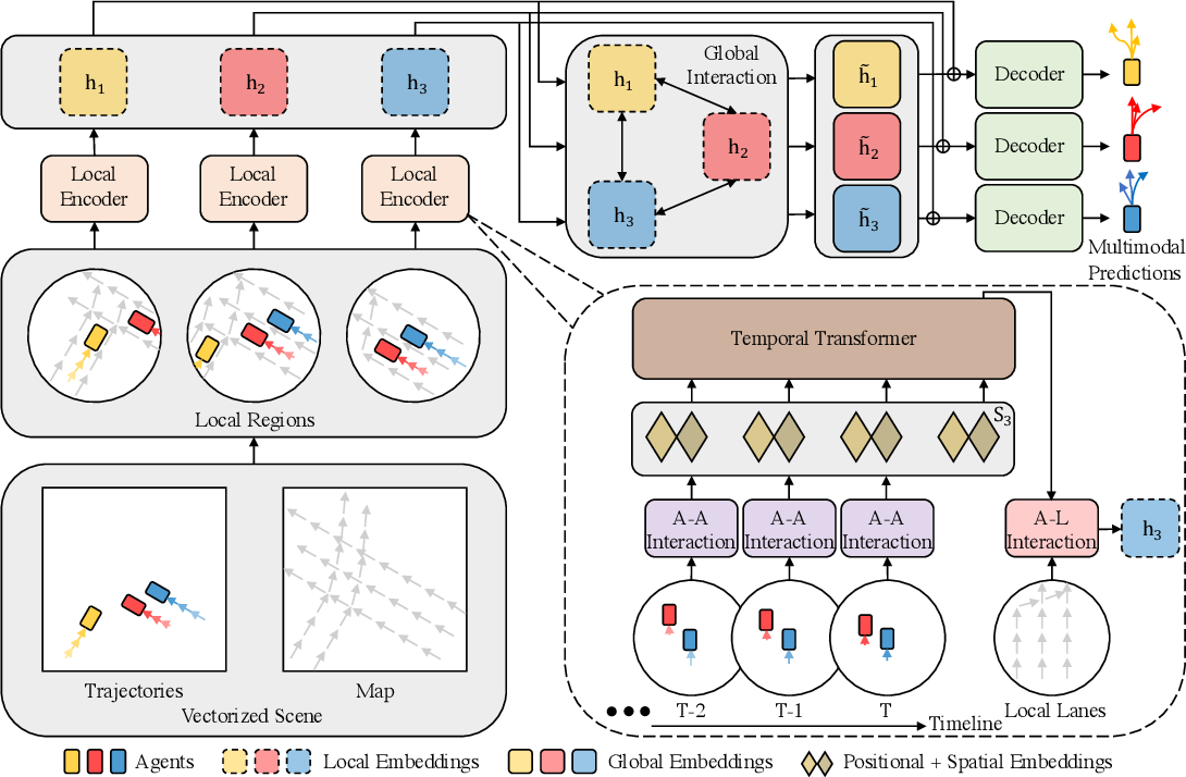
In the previous article, we got acquainted with the theoretical description of the Hierarchical Vector Transformer (HiVT) algorithm, which was proposed for multi-agent motion prediction for autonomous driving vehicles. This method offers an effective approach to solving the forecasting problem by decomposing the problem into stages of local context extraction and global interaction modeling.
Here's a brief overview of the method. The time series forecasting problem is solved by the authors of the HiVT method in 3 stages. In the first stage, the model extracts local contextual features of objects. The entire scene is divided into a set of local regions, each centered on a single central agent.
In the second stage, global long-range dependencies on the scene are recorded by transmitting information between agent-centered local areas.
The combined local and global representations enable the decoder to predict the future trajectories of all agents in a single forward pass of the model.
The author's visualization of the method is presented below.
In addition, in the previous article, we conducted quite extensive preparatory work, during which individual blocks of the proposed algorithm were implemented. In this article, we will complete the work we started, uniting the individual disparate blocks into a single complex structure.
1. Assembling HiVT
We will implement our vision of the approaches, that were proposed by HiVT authors, within the framework of the CNeuronHiVTOCL class. The core functionality will be inherited from the base fully connected layer class CNeuronBaseOCL. And its full structure is presented below.
class CNeuronHiVTOCL    :  public CNeuronBaseOCL
  {
protected:
   uint              iHistory;
   uint              iVariables;
   uint              iForecast;
   uint              iNumTraj;
   //---
   CNeuronBaseOCL               cDataTAD;
   CNeuronConvOCL               cEmbeddingTAD;
   CNeuronTransposeRCDOCL       cTransposeATD;
   CNeuronHiVTAAEncoder         cAAEncoder;
   CNeuronTransposeRCDOCL       cTransposeTAD;
   CNeuronLearnabledPE          cPosEmbeddingTAD;
   CNeuronMVMHAttentionMLKV     cTemporalEncoder;
   CNeuronLearnabledPE          cPosLineEmbeddingTAD;
   CNeuronPatching              cLineEmbeddibg;
   CNeuronMVCrossAttentionMLKV  cALEncoder;
   CNeuronMLMHAttentionMLKV     cGlobalEncoder;
   CNeuronTransposeOCL          cTransposeADT;
   CNeuronConvOCL               cDecoder[3]; // Agent * Traj * Forecast
   CNeuronConvOCL               cProbProj;
   CNeuronSoftMaxOCL            cProbability; // Agent * Traj
   CNeuronBaseOCL               cForecast;
   CNeuronTransposeOCL          cTransposeTA;
   //---
   virtual bool      Prepare(const CNeuronBaseOCL *history);
   //---
   virtual bool      feedForward(CNeuronBaseOCL *NeuronOCL) override ;
   //---
   virtual bool      calcInputGradients(CNeuronBaseOCL *NeuronOCL) override;
   virtual bool      updateInputWeights(CNeuronBaseOCL *NeuronOCL) override;

public:
                     CNeuronHiVTOCL(void) {};
                    ~CNeuronHiVTOCL(void) {};
   //---
   virtual bool      Init(uint numOutputs, uint myIndex, COpenCLMy *open_cl,
                          uint window, uint window_key, uint heads, uint units_count,
                          uint forecast, uint num_traj,
                          ENUM_OPTIMIZATION optimization_type, uint batch);
   //---
   virtual int       Type(void)   const   {  return defNeuronHiVTOCL; }
   //---
   virtual bool      Save(int const file_handle);
   virtual bool      Load(int const file_handle);
   //---
   virtual bool      WeightsUpdate(CNeuronBaseOCL *source, float tau);
   virtual void      SetOpenCL(COpenCLMy *obj);
  };
The presented structure of the CNeuronHiVTOCL object contains the declaration of the already familiar list of overridable methods and a whole series of internal objects, whose functionalities we will explore during the implementation of algorithms of the overridable methods.
We declare all internal objects as static and thus we can leave the class constructor and destructor empty. All nested objects and variables are initialized in the Init method.
bool CNeuronHiVTOCL::Init(uint numOutputs, uint myIndex, COpenCLMy *open_cl,

                          uint window, uint window_key, uint heads, uint units_count,
                          uint forecast, uint num_traj,
                          ENUM_OPTIMIZATION optimization_type, uint batch)
  {
   if(units_count < 2 ||
      !CNeuronBaseOCL::Init(numOutputs, myIndex, open_cl, window * forecast, optimization_type, batch))
      return false;
In the method parameters, we receive the main constants that allow us to uniquely identify the architecture of the initialized object. In the body of the method, we call the relevant method of the parent class. As you know, it implements the initialization of all inherited objects and variables.
Please note that we add a direct check of the number of elements in the analyzed sequence to the controls implemented in the parent class method. In this case, there must be at least 2 of them. This is because in the process of vectorization of the initial state, which is provided by the HiVT algorithm, we will operate with the value dynamics. Therefore, to calculate the change in the value, we need 2 references: at the current and previous time step.
After successfully passing the control block within the initialization method, we save the received parameters of the block architecture in local variables.
   iVariables = window;
   iHistory = units_count - 1;
   iForecast = forecast;
   iNumTraj = MathMax(num_traj, 1);
Next we initialize the internal objects. The order of initialization of internal objects will correspond to the sequence of use of objects within the feed-forward pass algorithm. This approach will allow us to once again work through the algorithm being constructed, as well as to ensure both the sufficiency and necessity of creating objects.
First, we will create an inner layer object to record the vector representation of the analyzed state of the environment.
Let me remind you that here the vector of description of each individual element of the univariate sequence at a separate time step is equal to twice the number of analyzed univariate sequences. Because each element of the sequence is characterized by movement in two-dimensional space and a change in the position of the remaining agents relative to the element being analyzed.
We create such a description vector for each element of all analyzed univariate sequences at each time step.
   if(!cDataTAD.Init(0, 0, OpenCL, 2 * iVariables * iVariables * iHistory, optimization, iBatch))
      return false;
Please note that when implementing the HiVT algorithm, we build work with three-dimensional tensors, saving their image in a one-dimensional data buffer. To indicate the current dimension in the names of objects, we add a 3-character suffix:
- T (Time) — the dimension of time steps;
- A (Agent) — the dimension of the agent (univariate time series); in our case it is the analyzed parameter;
- D (Dimension) — the dimension f the vector describing on element of the univariate sequence.
Next, we will use a convolutional layer to create embeddings of the resulting vector descriptions.
   if(!cEmbeddingTAD.Init(0, 1, OpenCL, 2 * iVariables, 2 * iVariables, window_key, iVariables * iHistory,
                                                                                  1, optimization, iBatch))
      return false;
In this case, to generate embeddings, we use 1 parameter matrix, which we apply to all elements of the multimodal sequence. Therefore, we will indicate the number of analyzed blocks of a given layer as the product of the number of univariate sequences by the depth of the analyzed history.
After generating embeddings, following the HiVT algorithm, we need to analyze local dependencies between agents within one time step. As discussed in the previous article, before performing this step, we need to transpose the original data.
   if(!cTransposeATD.Init(0, 2, OpenCL, iHistory, iVariables, window_key, optimization, iBatch))
      return false;
Only then can we use the attention classes to identify dependencies between agents in the local group.
   if(!cAAEncoder.Init(0, 3, OpenCL, window_key, window_key, heads, (heads + 1) / 2, iVariables, 2, 1,
                                                                       iHistory, optimization, iBatch))
      return false;
Please pay attention to the following two moments. First, after transposing the data, we modified the sequence of characters in the object name suffix to ATD, which corresponds to the dimensionality of the three-dimensional tensor at the output of the data transposition layer.
Second, let's examine the functionality of our attention blocks. Initially, they were designed to work with two-dimensional tensors, where each row represents the description vector of a single sequence element. Essentially, we identify dependencies between the rows of the analyzed matrix - performing what can be described as "vertical attention". Later, we introduced the detection of dependencies within individual univariate sequences of a multimodal time series. In practice, we divided the original matrix into several identical matrices, each containing fewer unitary series. These new matrices inherited the number of rows from the original matrix while their columns were evenly distributed among them. Structurally, this aligns with the dimensionality of our three-dimensional tensor. The first dimension represents the number of rows in the original data matrix. The second dimension indicates the number of smaller matrices used for independent analysis. The third dimension represents the size of the description vector for a single sequence element. Taking into account the prior transposition of the embedding tensor from the original data, we define the number of unitary sequences as the size of the analyzed sequence in the current attention block. Meanwhile, the depth of the analyzed historical data is specified in the parameter that represents the number of variables. This approach allows us to analyze dependencies between individual variables within a single time step.
In this implementation of the Agent-Agent dependency analysis block, I utilized two attention layers, generating a Key-Value tensor for each internal layer. The number of attention heads in the Key-Value tensor is half that of the equivalent parameter in the Query tensor.
Additionally, note that in this case, we use an attention block with the CNeuronHiVTAAEncoder feature management function.
After enriching the sequence element embeddings with dependencies between agents within a local group, the HiVT algorithm provides for the analysis of temporal dependencies within individual unitary sequences. At this stage, we need to return the data to its original representation.
   if(!cTransposeTAD.Init(0, 4, OpenCL, iVariables, iHistory, window_key, optimization, iBatch))
      return false;
Then we add fully trainable positional encoding.
   if(!cPosEmbeddingTAD.Init(0, 5, OpenCL, iVariables * iHistory * window_key, optimization, iBatch))
      return false;
Next, we use the attention block CNeuronMVMHAttentionMLKV to identify temporal dependencies.
   if(!cTemporalEncoder.Init(0, 6, OpenCL, window_key, window_key, heads, (heads + 1) / 2, iHistory, 2, 1,
                                                                          iVariables, optimization, iBatch))
      return false;
Despite the differences in the architecture of the local and temporal dependency attention blocks, we use the same parameters to initialize them.
In the next step, HiVT authors propose to enrich Agents embeddings with the information about the roadmap. I think no one doubts that the condition of the road, its markings and bends leave a certain imprint on the agent's actions. In our case, there are no clear guidelines for limiting changes in the values of the analyzed parameters. Of course, there are areas of acceptable values for individual oscillators. For example RSI can only take values in the range from 0 to 100. But this is an isolated case.
So we'll use the historical data we have to determine the most likely change. We will replace the roadmap representation with embeddings of actual small segments of trajectories, which we will create using a data patching layer.
   if(!cLineEmbeddibg.Init(0, 7, OpenCL, 3, 1, 8, iHistory - 1, iVariables, optimization, iBatch))
      return false;
Note that when vectorizing the current state, we used the dynamics of the parameter change over 1 time step. But when embedding actual small sections of the trajectory, we use blocks of 3 elements with a step of 1. In this way, we want to identify the dependencies between the dynamics of the indicator at a particular step and the possible continuation of the trajectory.
Then we add fully trainable positional encoding to the resulting embeddings.
   if(!cPosLineEmbeddingTAD.Init(0, 8, OpenCL, cLineEmbeddibg.Neurons(), optimization, iBatch))
      return false;
Then we enrich the current Agent embeddings with information about trajectories. For this, we use the cross-attention block CNeuronMVCrossAttentionMLKV with two inner layers.
   if(!cALEncoder.Init(0, 9, OpenCL, window_key, window_key, heads, 8, (heads + 1) / 2,
                       iHistory, iHistory - 1, 2, 1, iVariables, iVariables, optimization, iBatch))
      return false;
It may seem here that we are sequentially performing two similar operations: identifying temporal dependencies and analyzing dependencies between agents and trajectories. In both cases, we analyze the dependencies of the current state of the Agent with the representation of the parameters of the same indicator at other time intervals. But there is a fine line here. In the first case, we compare similar states of the agent at separate time steps. In the second case, we are dealing with certain trajectory patterns that cover a slightly larger time interval.
This completes the local dependency analysis block, which essentially enriches the Agent state embedding in a comprehensive manner. The next step of the HiVT algorithm is the analysis of long-term dependencies of the scene in the global interaction block.
   if(!cGlobalEncoder.Init(0, 10, OpenCL, window_key*iVariables, window_key*iVariables, heads, (heads+1)/2,
                                                                      iHistory, 4, 2, optimization, iBatch))
      return false;
Here we use an attention block with 4 internal layers. To analyze dependencies, we use a representation not of individual Agents, but of the entire scene.
Then we need to model the upcoming sequence of predicted values. As before, the prediction of the upcoming sequence is implemented within the framework of individual univariate sequences. To do this, we first need to transpose the current data.
   if(!cTransposeADT.Init(0, 11, OpenCL, iHistory, window_key * iVariables, optimization, iBatch))
      return false;
Further, to predict subsequent values for the entire planning depth, the authors of the HiVT method suggest using an MLP. In our case, this work is performed in a block of 3 consecutive convolutional layers, each of which received a unique window of analyzed data and its own activation function.
   if(!cDecoder[0].Init(0, 12, OpenCL, iHistory, iHistory, iForecast, window_key * iVariables,
                                                                                         optimization, iBatch))
      return false;
   cDecoder[0].SetActivationFunction(SIGMOID);
   if(!cDecoder[1].Init(0, 13, OpenCL, iForecast * window_key, iForecast * window_key, iForecast * window_key,
                                                                             iVariables, optimization, iBatch))
      return false;
   cDecoder[1].SetActivationFunction(LReLU);
   if(!cDecoder[2].Init(0, 14, OpenCL, iForecast * window_key, iForecast * window_key, iForecast * iNumTraj,
                                                                             iVariables, optimization, iBatch))
      return false;
   cDecoder[2].SetActivationFunction(TANH);
In the first stage, we work within the framework of individual elements of the embedding description of the state of an individual Agent, changing the size of the sequence from the depth of the analyzed history to the planning horizon.
We then analyze global dependencies within individual agents over the entire planning horizon without changing the tensor size.
Only in the last stage do we predict several possible scenarios for each individual univariate time series. The number of variants of predicted trajectories is specified by an external program in the method parameters.
It should be noted here that forecasting several possible scenarios is a distinctive feature of the proposed approach. However, we need a mechanism to select the most probable trajectory. Therefore, we first project the obtained trajectories to the dimension of the number of predicted trajectories for each agent.
   if(!cProbProj.Init(0, 15, OpenCL, iForecast * iNumTraj, iForecast * iNumTraj, iNumTraj, iVariables,
                                                                                 optimization, iBatch))
      return false;
Then we use a SoftMax function to translate the obtained projections into the probability domain.
   if(!cProbability.Init(0, 16, OpenCL, iForecast * iNumTraj * iVariables, optimization, iBatch))
      return false;
   cProbability.SetHeads(iVariables); // Agent * Traj
By weighing previously predicted trajectories by their probabilities, we obtain the average trajectory of the upcoming movement of our Agent.
   if(!cForecast.Init(0, 17, OpenCL, iForecast * iVariables, optimization, iBatch))
      return false;
Now, we just need to convert the predicted values to the dimensions of the original data. We implement functionality by transposing data.
   if(!cTransposeTA.Init(0, 18, OpenCL, iVariables, iForecast, optimization, iBatch))
      return false;
In order to reduce data copy operations and optimize memory resource usage, we redefine the result and error gradient buffer pointers of our block to similar buffers of the last internal data transposition layer.
   SetOutput(cTransposeTA.getOutput(),true);
   SetGradient(cTransposeTA.getGradient(),true);
//---
   return true;
  }
Then we complete the method operation by returning the logical result of the method operations to the calling program.
After completing the work on initializing the class object, we move on to building the feed-forward algorithm for our class in the feedForward method.
bool CNeuronHiVTOCL::feedForward(CNeuronBaseOCL *NeuronOCL)
  {
   if(!Prepare(NeuronOCL))
      return false;
In the method parameters, we receive a pointer to an object containing the original data. We immediately pass the received pointer to the Prepare method that prepares the initial data. This method is a "wrapper" for calling the data vectorization kernel HiVTPrepare. We discussed its algorithm in the previous article. We have already looked at various methods for queuing OpenCL program kernels. The algorithm of the Prepare method does not have any special features. Therefore, I will omit the description of its algorithm in this article. You can study it independently using the code provided in the attachment.
Next, based on the obtained vector representations, we generate Agent embeddings at each individual time step.
   if(!cEmbeddingTAD.FeedForward(cDataTAD.AsObject()))
      return false;
We transpose them.
   if(!cTransposeATD.FeedForward(cEmbeddingTAD.AsObject()))
      return false;
And then we enrich local dependencies within the framework of the analysis of Agent-Agent representations.
   if(!cAAEncoder.FeedForward(cTransposeATD.AsObject()))
      return false;
In the next step, we enrich the agent state embeddings by adding temporal dependencies. To do this, we first transpose the current data tensor.
   if(!cTransposeTAD.FeedForward(cAAEncoder.AsObject()))
      return false;
We add positional encoding marks to it.
   if(!cPosEmbeddingTAD.FeedForward(cTransposeTAD.AsObject()))
      return false;
And then we call the feed-forward method of our temporal attention module in the context of individual agents.
   if(!cTemporalEncoder.FeedForward(cPosEmbeddingTAD.AsObject()))
      return false;
After successful execution of temporal attention operations, we obtain a tensor of embeddings of the analyzed data, enriched with local and temporal dependencies. Now we need to enrich the resulting embeddings with information about possible movement patterns. To do this, we first create embeddings of the patterns of the historical movement being analyzed.
   if(!cLineEmbeddibg.FeedForward(NeuronOCL))
      return false;
We add positional coding to the resulting pattern embeddings.
   if(!cPosLineEmbeddingTAD.FeedForward(cLineEmbeddibg.AsObject()))
      return false;
In the cross-attention module, we enrich our agents' embeddings with information about various movement patterns.
   if(!cALEncoder.FeedForward(cTemporalEncoder.AsObject(), cPosLineEmbeddingTAD.getOutput()))
      return false;
We apply the global attention module to the tensor of enriched agent embeddings.
   if(!cGlobalEncoder.FeedForward(cALEncoder.AsObject()))
      return false;
This is followed by a block of forecasting the upcoming agent movement. Let me remind you that we plan to forecast subsequent values of the analyzed parameters in terms of univariate sequences. Therefore, we first transpose the given data tensor.
   if(!cTransposeADT.FeedForward(cGlobalEncoder.AsObject()))
      return false;
Next, we run a feed-forward pass of our three-layer MLP block for data prediction.
   if(!cDecoder[0].FeedForward(cTransposeADT.AsObject()))
      return false;
   if(!cDecoder[1].FeedForward(cDecoder[0].AsObject()))
      return false;
   if(!cDecoder[2].FeedForward(cDecoder[1].AsObject()))
      return false;
Here we should remember the peculiarity of the HiVT method. The MLP forecasting the upcoming movement outputs not one but several variants for the possible continuation of the analyzed initial series. We have to determine the probabilities of each variant of the predicted movement. To do this, we will first make predictive trajectories.
   if(!cProbProj.FeedForward(cDecoder[2].AsObject()))
      return false;
Using the SoftMax function, we translate the obtained projections into the probability domain.
   if(!cProbability.FeedForward(cProbProj.AsObject()))
      return false;
Now we just need to multiply the tensor of predicted trajectories by their probabilities.
   if(IsStopped() ||
      !MatMul(cDecoder[2].getOutput(), cProbability.getOutput(), cForecast.getOutput(), iForecast,
                                                                          iNumTraj, 1, iVariables))
      return false;
As a result of this operation, we obtain a tensor of average-weighted trajectories for the entire planning horizon for each univariate series of the analyzed multimodal sequence.
At the end of our feed-forward method operations, we transpose the predicted value tensor to match the measurements of the original data.
   if(!cTransposeTA.FeedForward(cForecast.AsObject()))
     return false;
//---
   return true;
  }
As usual, we return a Boolean value to the calling program, indicating the success of the method operations.
With this, we conclude the implementation of the forward pass algorithm for the HiVT method and move on to developing the backward pass methods for our class. As you know, the backward pass algorithm consists of two main components:
- Gradient error distribution to all elements based on their influence on the final result. This functionality is implemented in the calcInputGradients method.
- Adjustment of trainable model parameters to minimize the overall loss, which is carried out in the updateInputWeights method.
We will begin the implementation of the backward pass algorithms by developing the gradient error distribution method, calcInputGradients. The logic of this method fully mirrors that of the forward pass algorithm, except that all operations are performed in reverse order.
bool CNeuronHiVTOCL::calcInputGradients(CNeuronBaseOCL *NeuronOCL)
  {
   if(!NeuronOCL)
      return false;
As input parameters, this method receives a pointer to the previous layer's object - the same layer that provided the input data during the feed-forward pass. However, in this case, we need to pass the error gradient back to it, ensuring that it reflects the influence of the original input data on the final result.
In the body of the method, we immediately check the relevance of the received pointer. If the pointer is invalid, executing the method operations would be meaningless.
Once the validation checks are successfully passed, we proceed to distribute the error gradient accordingly.
At the current layer's output level, the error gradient is already stored in the corresponding buffer of our class. It was recorded there during the execution of the equivalent method in the subsequent layer. Due to the previously implemented buffer swapping mechanism, the required error gradient is already available in the buffer of the final data transposition layer. From here, we begin propagating the error gradient to the level of the weighted average forecast trajectory layer for univariate time series.
   if(!cForecast.calcHiddenGradients(cTransposeTA.AsObject()))
      return false;
As you remember, in the feed-forward pass we obtained the weighted average trajectories by multiplying the tensor of several predicted trajectories by the vector of the corresponding probabilities. Accordingly, in the process of the backpropagation pass, we have to distribute the error gradient both on the tensor of the set of predicted trajectories and on the probability vector.
   if(IsStopped() ||
      !MatMulGrad(cDecoder[2].getOutput(), cDecoder[2].getGradient(), cProbability.getOutput(),
                  cProbability.getGradient(), cForecast.getGradient(), iForecast, iNumTraj, 1, iVariables))
      return false;
We will pass the probability error gradient to the projection layer of predicted trajectories.
   if(!cProbProj.calcHiddenGradients(cProbability.AsObject()))
      return false;
To obtain projections, we used the forecast trajectories themselves. Following this, we would typically pass the error gradient to the forecast trajectory level.
However, it is important to note that the error gradient for the set of forecast trajectories has already been passed from the weighted average trajectory at the previous step. A direct call of the calcHiddenGradients method of the corresponding layer would overwrite the previously transferred error gradient, replacing the buffer with new values. In such cases, we typically use auxiliary data buffers, summing values from two data streams to preserve all information. However, in this particular instance, a decision was made not to pass the error gradient further into the data projection layer. The goal of this approach is to keep the forecasting of subsequent trajectories "clean", preventing distortions caused by the probabilistic distribution errors associated with the relevance of individual trajectories.
Instead, we propagate the error gradient of the forecast trajectories through the MLP layer of the forecasting block.
   if(!cDecoder[1].calcHiddenGradients(cDecoder[2].AsObject()))
      return false;
   if(!cDecoder[0].calcHiddenGradients(cDecoder[1].AsObject()))
      return false;
We transpose the resulting error gradient tensor and pass it through the global interaction block.
   if(!cTransposeADT.calcHiddenGradients(cDecoder[0].AsObject()))
      return false;
   if(!cGlobalEncoder.calcHiddenGradients(cTransposeADT.AsObject()))
      return false;
   if(!cALEncoder.calcHiddenGradients(cGlobalEncoder.AsObject()))
      return false;
From the global interaction block, the error gradient is then passed to the local dependency analysis block.
As a reminder, this block performs a comprehensive analysis of mutual dependencies between individual local objects. Here, we first pass the received error gradient through the Agent-Trajectory cross-attention block, down to the level of temporal dependency analysis and positional encoding of motion pattern embeddings.
   if(!cTemporalEncoder.calcHiddenGradients(cALEncoder.AsObject(), cPosLineEmbeddingTAD.getOutput(),
                                                                   cPosLineEmbeddingTAD.getGradient(),
                                                  (ENUM_ACTIVATION)cPosLineEmbeddingTAD.Activation()))
      return false;
We propagate the error gradient through positional coding operations.
   if(!cLineEmbeddibg.calcHiddenGradients(cPosLineEmbeddingTAD.AsObject()))
      return false;
And then we pass it to the source data level.
   if(!NeuronOCL.calcHiddenGradients(cLineEmbeddibg.AsObject()))
      return false;
For the second data stream, we first propagate the error gradient through the temporal dependency analysis block.
   if(!cPosEmbeddingTAD.calcHiddenGradients(cTemporalEncoder.AsObject()))
      return false;
After that, we adjust the obtained error gradient in the positional coding operation.
   if(!cTransposeTAD.calcHiddenGradients(cPosEmbeddingTAD.AsObject()))
      return false;
Then we transpose the data and propagate the gradient through the Agent-Agent dependency analysis block.
   if(!cAAEncoder.calcHiddenGradients(cTransposeTAD.AsObject()))
      return false;
   if(!cTransposeATD.calcHiddenGradients(cAAEncoder.AsObject()))
      return false;
At the end of the method operations, we transpose the data into the original representation and propagate the error gradient through the embedding generation layer to the vector representation of the original data.
   if(!cEmbeddingTAD.calcHiddenGradients(cTransposeATD.AsObject()))
      return false;
   if(!cDataTAD.calcHiddenGradients(cEmbeddingTAD.AsObject()))
      return false;
//---
   return true;
  }
As usual, we return a Boolean value to the calling program, indicating the execution result of the method operations.
At this stage, we have distributed the error gradient to all model elements according to their influence on the final result. Now, we need to adjust the trainable model parameters to minimize the overall error. This functionality is implemented in the updateInputWeights method.
It is important to note that all trainable parameters of our new class CNeuronHiVTOCL are stored within its internal objects. However, not all internal objects contain trainable parameters. For example, the data transposition layers do not include them. Therefore, in this method, we only interact with objects that contain trainable parameters. To adjust them, it is sufficient to call the corresponding method of each internal object.
As you can see, the logic of this method is quite simple, so we will not provide its full code in this article. You can study it independently using the code provided in the attachment. The attachments also include the complete source code of our new class and all its methods.
2. Model architecture
We have completed the development of the CNeuronHiVTOCL class and its methods. The class implements our interpretation of the approaches proposed by the authors of the HiVT method. Now, it is time to integrate the new object into the architecture of our model.
As before, we incorporate the forecasting object for future movement of the analyzed multimodal series into the Environmental State Encoder model. The architectural design of this model is defined in the CreateEncoderDescriptions method. This method receives a pointer to a dynamic array object, where we record the architecture of the generated model.
bool CreateEncoderDescriptions(CArrayObj *&encoder)
  {
//---
   CLayerDescription *descr;
//---
   if(!encoder)
     {
      encoder = new CArrayObj();
      if(!encoder)
         return false;
     }
In the method body, we check the relevance of the received pointer and, if necessary, create a new instance of the dynamic array. After that, we move on to a sequential description of the architectural solution of each layer of our model.
To obtain the initial data, we use a fully connected base layer of sufficient size.
//--- Encoder
   encoder.Clear();
//--- Input layer
   if(!(descr = new CLayerDescription()))
      return false;
   descr.type = defNeuronBaseOCL;
   int prev_count = descr.count = (HistoryBars * BarDescr);
   descr.activation = None;
   descr.optimization = ADAM;
   if(!encoder.Add(descr))
     {
      delete descr;
      return false;
     }
We plan to input raw, unprocessed data into the model. To bring such data into a comparable form, we use batch normalization layers.
//--- layer 1
   if(!(descr = new CLayerDescription()))
      return false;
   descr.type = defNeuronBatchNormOCL;
   descr.count = prev_count;
   descr.batch = 1e4;
   descr.activation = None;
   descr.optimization = ADAM;
   if(!encoder.Add(descr))
     {
      delete descr;
      return false;
     }
After the initial processing, we immediately transfer the original data to our new block, built using the approaches of the HiVT method.
//--- layer 2
   if(!(descr = new CLayerDescription()))
      return false;
   descr.type = defNeuronHiVTOCL;
     {
      int temp[] = {BarDescr, NForecast, 6};          // {Variables, Forecast, NumTraj}
      ArrayCopy(descr.windows, temp);
     }
   descr.window_out = EmbeddingSize;                  // Inside Dimension
   descr.count = HistoryBars;                         // Units
   descr.batch = 1e4;
   descr.activation = None;
   descr.optimization = ADAM;
   if(!encoder.Add(descr))
     {
      delete descr;
      return false;
     }
Here we practically repeat similar parameters from previous works. Only 1 new block parameter is added, which determines the number of variants of predicted trajectories. In this case, we use 6.
At the output of the CNeuronHiVTOCL block, we expect to receive ready-made forecast values of the analyzed multimodal time series. But there is one caveat. To organize the efficient operation of the model with a multimodal time series, we brought all its values into a comparable form. Accordingly, we obtained the predicted values in a similar form. To bring the obtained forecast values into line with the usual values of the original data, we will add to them the statistical parameters of the distribution that were removed during the normalization of the raw data.
//--- layer 3
   if(!(descr = new CLayerDescription()))
      return false;
   descr.type = defNeuronRevInDenormOCL;
   descr.count = BarDescr * NForecast;
   descr.activation = None;
   descr.optimization = ADAM;
   descr.layers = 1;
   if(!encoder.Add(descr))
     {
      delete descr;
      return false;
     }
After that, we will coordinate the obtained results in the frequency domain.
//--- layer 4
   if(!(descr = new CLayerDescription()))
      return false;
   descr.type = defNeuronFreDFOCL;
   descr.window = BarDescr;
   descr.count =  NForecast;
   descr.step = int(true);
   descr.probability = 0.7f;
   descr.activation = None;
   descr.optimization = ADAM;
   if(!encoder.Add(descr))
     {
      delete descr;
      return false;
     }
//---
   return true;
  }
The architectures of the Actor and Critic models remain unchanged. The same can be said about model training programs. Therefore, we will not discuss them in detail within the framework of this article. However, the full source code of all programs used in this study is available in the attached materials for further exploration.
3. Testing
We have completed the implementation of our interpretation of the HiVT method. Now it is time to evaluate the effectiveness of our solutions. First, we need to train the models on real historical data and then test the trained models on a dataset that was not part of the training set.
For training, we use historical EURUSD data on the H1 timeframe for the entire year 2023.
Training is conducted offline. Therefore, we first need to compile the required training dataset. More details on this process can be found in our article on the Real-ORL method. For training our Environmental State Encoder, we used a dataset collected during the operation of previous models.
As you know, the State Encoder model works only with historical price movement data and analyzed indicators, which are independent of the Agent's actions. Therefore, at this stage, it is not necessary to periodically update the training dataset, as newly added trajectories do not provide additional information for the Encoder. We continue the training process until we achieve the desired results.
The results of the trained model's testing are presented below.
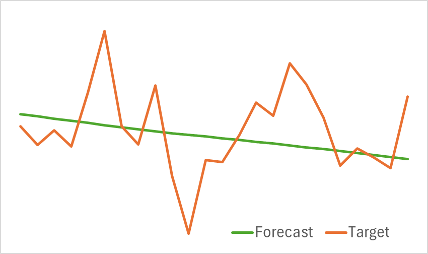
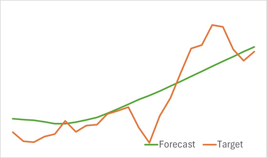
As can be seen from the provided graphs, our model effectively captures key trends in upcoming price movements.
Next, we proceed to the second stage of training, which focuses on training the Actor's profit-maximizing behavior policy and the Critic's reward function. Unlike the Encoder, the Actor's training depends significantly on the actions it takes within the environment. To ensure effective learning, we must keep the training dataset up to date. Therefore, we periodically update the dataset to reflect the Actor's current policy.
The training continues until the model's error stabilizes at a certain level. At which point further dataset updates no longer contribute to optimizing the Actor's policy.
We evaluate the effectiveness of the trained model using the MetaTrader 5 strategy tester, applying historical data from January 2024, while keeping all other parameters unchanged. The results of the trained model's testing are presented below.
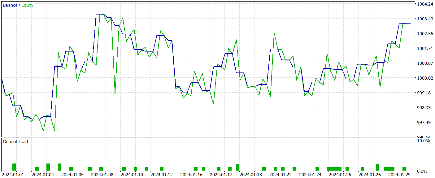
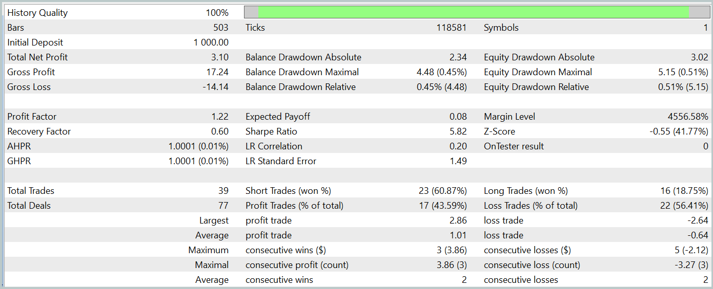
As the results indicate, our training process successfully produced an Actor policy capable of generating profits on both training and test data. During the testing period, the model executed 39 trades, with over 43% of them closing in profit. The proportion of profitable trades was slightly lower than losing trades. However, the average and maximum profit per trade exceeded the corresponding losses, allowing the model to finish testing with a small net profit. The profit factor was recorded at 1.22.
However, it is important to note that due to the lack of a clear trend in the observed balance line and the limited number of trades, the obtained results may not be fully representative.
Conclusion
In this article, we successfully implemented the HiVT method using MQL5. We integrated the proposed algorithm into the Environmental State Encoder model. We then proceeded with training and testing the models. The test results demonstrated that the HiVT method effectively captures market trends. It also provided a sufficient level of prediction quality to support the development of a profitable trading policy for the Agent.
References
Programs used in the article
| # | Issued to | Type | Description |
|---|---|---|---|
| 1 | Research.mq5 | Expert Advisor | EA for collecting examples |
| 2 | ResearchRealORL.mq5 | Expert Advisor | EA for collecting examples using the Real-ORL method |
| 3 | Study.mq5 | Expert Advisor | Model training EA |
| 4 | StudyEncoder.mq5 | Expert Advisor | Encoder training EA |
| 5 | Test.mq5 | Expert Advisor | Model testing EA |
| 6 | Trajectory.mqh | Class Library | System state description structure |
| 7 | NeuroNet.mqh | Class Library | A library of classes for creating a neural network |
| 8 | NeuroNet.cl | Library | OpenCL program code library |
Translated from Russian by MetaQuotes Ltd.
Original article: https://www.mql5.com/ru/articles/15713
Warning: All rights to these materials are reserved by MetaQuotes Ltd. Copying or reprinting of these materials in whole or in part is prohibited.
This article was written by a user of the site and reflects their personal views. MetaQuotes Ltd is not responsible for the accuracy of the information presented, nor for any consequences resulting from the use of the solutions, strategies or recommendations described.

- Free trading apps
- Over 8,000 signals for copying
- Economic news for exploring financial markets
You agree to website policy and terms of use