Neural Networks in Trading: Exploring the Local Structure of Data

Introduction

The task of object detection in point clouds is gaining increasing attention. The effectiveness of solving this task heavily depends on the information about the structure of local regions. However, the sparse and irregular nature of point clouds often results in incomplete and noisy local structures.

Traditional convolution-based object detection relies on fixed kernels, treating all neighboring points equally. As a result, unrelated or noisy points from other objects are inevitably included in the analysis.

The Transformer has proven its effectiveness in addressing various tasks. Compared to convolution, the Self-Attention mechanism can adaptively filter out noisy or irrelevant points. Nevertheless, the vanilla Transformer applies the same transformation function to all elements in a sequence. This isotropic approach disregards spatial relationships and local structure information such as direction and distance from a central point to its neighbors. If the positions of the points are rearranged, the output of the Transformer remains unchanged. This creates challenges in recognizing the directionality of objects, which is crucial for detecting price patterns.

The authors of the paper "SEFormer: Structure Embedding Transformer for 3D Object Detection" aimed to combine the strengths of both approaches by developing a new transformer architecture - Structure-Embedding transFormer (SEFormer), capable of encoding local structure with attention to direction and distance. The proposed SEFormer learns distinct transformations for the Value of points from different directions and distances. Consequently, changes in the local spatial structure are reflected in the model's output, providing a key to accurate recognition of object directionality.

Based on the proposed SEFormer module, the study introduces a multi-scale network for 3D object detection.

1. The SEFormer Algorithm

Locality and spatial invariance of convolution align well with the inductive bias in image data. Another key advantage of convolution is its ability to encode structural information within the data. The authors of the SEFormer method decompose convolution into a two-step operation: transformation and aggregation. During the transformation step, each point is multiplied by a corresponding kernel wδ. These values are then simply summed with a fixed aggregation coefficient α=1. In convolution, kernels are learned differently depending on their directions and distances from the kernel center. As a result, convolution is capable of encoding the local spatial structure. However, during aggregation, all neighboring points are treated equally (α=1). The standard convolution operator uses a static and rigid kernel, but point clouds are often irregular and even incomplete. Consequently, convolution inevitably incorporates irrelevant or noisy points into the resulting feature.

Compared to convolution, the Self-Attention mechanism in Transformer provides a more effective method for preserving irregular shapes and object boundaries in point clouds. For a point cloud consisting of N elements 𝒑=[p1,…, pN], the Transformer computes the response for each point as follows:

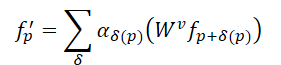
Here αδ represents the self-attention coefficients between points in the local neighborhood, while 𝑾v denotes the Value transformation. Compared to static α=1 in convolution, self-attention coefficients allow for the adaptive selection of points for aggregation, effectively excluding the influence of unrelated points. However, the same Value transformation is applied to all points in the Transformer, meaning it lacks the structural encoding capability inherent to convolution.

Given the above, the authors of SEFormer observed that convolution is capable of encoding data structure, while Transformers are effective at preserving it. Therefore, the straightforward idea is to develop a new operator that combines the advantages of both convolution and Transformer. This led to the proposal of SEFormer, which can be formulated as:

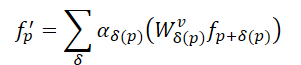
The key distinction between SEFormer and the vanilla Transformer lies in the Value transformation function, which is learned based on the relative positions of the points.

Given the irregularity of point clouds, the authors of SEFormer follow the Point Transformer paradigm, independently sampling neighboring points around each Query point before passing them into the Transformer. In their method, the authors opted to use grid interpolation to generate key points. Around each analyzed point, multiple virtual points are generated, arranged on a predefined grid. The distance between two grid elements is fixed at d.

These virtual points are then interpolated using their nearest neighbors in the analyzed point cloud. Compared to traditional sampling methods such as K-Nearest Neighbors (KNN), the advantage of grid sampling lies in its ability to enforce point selection from different directions. Grid interpolation enables a more precise representation of the local structure. However, since a fixed distance d is used for grid interpolation, the authors adopt a multi-radius strategy to enhance sampling flexibility.

SEFormer constructs a memory pool containing multiple Value transformation matrices (𝑾v). The interpolated key points search for their corresponding 𝑾v based on their relative coordinates with respect to the original point. As a result, their features are transformed differently. This enables SEFormer to encode structural information — a capability lacking in the vanilla Transformer.

In the object detection model proposed by the authors, a backbone based on 3D convolution is first constructed to extract multi-scale voxel features and generate initial proposals. The convolutional backbone transforms the raw input into a set of voxel features with downsampling factors of 1×, 2×, 4×, and 8×. These features of varying scales are processed at different depth levels. After feature extraction, the 3D volume is compressed along the Z-axis and converted into a 2D bird's-eye-view (BEV) feature map. These BEV maps are then used for generating initial candidate object predictions.

Next, the proposed spatial modulation structure aggregates the multi-scale features [𝑭1, 𝑭2, 𝑭3, 𝑭4] into several point-level embeddings 𝑬. Starting with 𝑬init, key points are interpolated from the smallest-scale feature map 𝑭1 for each analyzed element. The authors employ m different grid distances d to generate multi-scale sets of key features denoted as 𝑭1,1, 𝑭2,1,…, 𝑭m,1. This multi-radius strategy enhances the model's ability to handle the sparse and irregular distribution of point clouds. Then m parallel SEFormer blocks are applied to generate m updated embeddings 𝑬1,1, 𝑬2,1,…, 𝑬m,1. These embeddings are concatenated and transformed into a unified embedding 𝑬1 using a vanilla Transformer. 𝑬1 then repeats the previously described process and aggregates [𝑭2, 𝑭3, 𝑭4] into the final embedding 𝑬final. Compared to the original voxel features 𝑭, the final embedding 𝑬final offers a more detailed structural representation of the local area.

Based on the resulting point-level embeddings 𝑬final​, the model head proposed by the authors aggregates them into several object-level embeddings to produce the final object proposals. More specifically, each initial-stage proposal is divided into multiple cubic subregions, each of which is interpolated with the surrounding point-level object embeddings. Due to the sparsity of the point cloud, some regions are often empty. Traditional approaches simply sum features from non-empty regions. In contrast, SEFormer is capable of leveraging information from both populated and empty regions. The enhanced structural embedding capabilities of SEFormer allow for a richer object-level structural representation, thereby generating more accurate proposals.

The author's visualization of the method is presented below.

2. Implementation in MQL5

After reviewing the theoretical aspects of the proposed SEFormer method, we now move to the practical part of our paper, where we implement our interpretation of the suggested approaches. Let us begin by considering the architecture of our future model.

For initial feature extraction, the authors of the SEFormer method propose using voxel-based 3D convolution. In our case, however, the feature vector of a single bar may contain significantly more attributes. As such, this approach appears to be less efficient for our purposes. Therefore, I propose relying on our previously used approach, which aggregates features using a sparse attention block with varying attention concentration levels.

The second point worth highlighting is the construction of a grid around the analyzed point. In the 3D object detection task addressed by the SEFormer authors, the data can be compressed along the height dimension, allowing for analysis of objects on flat maps. In our case, however, the data representation is multidimensional, and each dimension can play a crucial role at any given moment. We cannot afford to compress the data along any single dimension. Moreover, constructing a "grid" in a high-dimensional space presents a considerable challenge. The number of elements increases geometrically with the number of features being analyzed. In my view, a more effective solution in this scenario is to let the model learn the most optimal centroid points in the multidimensional space.

In light of the above, I propose building our new object by inheriting the core functionality from the CNeuronPointNet2OCL class. The general structure of the new class CNeuronSEFormer is presented below.

class CNeuronSEFormer   :    public CNeuronPointNet2OCL
  {
protected:
   uint              iUnits;
   uint              iPoints;
   //---
   CLayer            cQuery;
   CLayer            cKey;
   CLayer            cValue;
   CLayer            cKeyValue;
   CArrayInt         cScores;
   CLayer            cMHAttentionOut;
   CLayer            cAttentionOut;
   CLayer            cResidual;
   CLayer            cFeedForward;
   CLayer            cCenterPoints;
   CLayer            cFinalAttention;
   CNeuronMLCrossAttentionMLKV SEOut;
   CBufferFloat      cbTemp;
   //---
   virtual bool      feedForward(CNeuronBaseOCL *NeuronOCL) override;
   virtual bool      AttentionOut(CBufferFloat *q, CBufferFloat *kv, int scores, CBufferFloat *out);
   virtual bool      AttentionInsideGradients(CBufferFloat *q, CBufferFloat *q_g,
                                              CBufferFloat *kv, CBufferFloat *kv_g,
                                              int scores, CBufferFloat *gradient);
   //---
   virtual bool      calcInputGradients(CNeuronBaseOCL *NeuronOCL) override;
   virtual bool      updateInputWeights(CNeuronBaseOCL *NeuronOCL) override;
   //---

public:
                     CNeuronSEFormer(void) {};
                    ~CNeuronSEFormer(void) {};
   //---
   virtual bool      Init(uint numOutputs, uint myIndex, COpenCLMy *open_cl,
                          uint window, uint units_count, uint output, bool use_tnets,
                          uint center_points, uint center_window,
                          ENUM_OPTIMIZATION optimization_type, uint batch);
   //---
   virtual int       Type(void) override   const   {  return defNeuronSEFormer; }
   //---
   virtual bool      Save(int const file_handle) override;
   virtual bool      Load(int const file_handle) override;
   //---
   virtual bool      WeightsUpdate(CNeuronBaseOCL *source, float tau) override;
   virtual void      SetOpenCL(COpenCLMy *obj) override;
  };

In the structure presented above, we can already see a familiar list of overridable methods and a number of nested objects. The names of some of these components may remind us of the Transformer architecture - and that's no coincidence. The authors of the SEFormer method aimed to enhance the vanilla Transformer algorithm. But first things first.

All internal objects of our class are declared statically, allowing us to leave the constructor and destructor empty. Initialization of both declared and inherited components is handled in the Init method, whose parameters, as you know, contain the core constants that define the architecture of the object being created.

bool CNeuronSEFormer::Init(uint numOutputs, uint myIndex, COpenCLMy *open_cl,
                           uint window, uint units_count, uint output, bool use_tnets,
                           uint center_points, uint center_window,
                           ENUM_OPTIMIZATION optimization_type, uint batch)
  {
   if(!CNeuronPointNet2OCL::Init(numOutputs, myIndex, open_cl, window, units_count, output, use_tnets,
                                 optimization_type, batch))
      return false;

In addition to the parameters we're already familiar with, we now introduce the number of trainable centroids and the dimensionality of the vector representing their state.

It's important to note that the architecture of our block is designed in such a way that the dimensionality of the centroid's descriptor vector can differ from the number of features used to describe a single analyzed bar.

Within the method body, as usual, we begin by calling the corresponding method of the parent class, which already implements the mechanisms for parameter validation and initialization of inherited components. We simply verify the logical result of the parent method's execution.

After that, we store several architecture parameters that will be required during the execution of the algorithm being constructed.

   iUnits = units_count;
   iPoints = MathMax(center_points, 9);

As an array of internal objects, I used CLayer objects. To enable their correct operation, we pass a pointer to the OpenCL context object.

   cQuery.SetOpenCL(OpenCL);
   cKey.SetOpenCL(OpenCL);
   cValue.SetOpenCL(OpenCL);
   cKeyValue.SetOpenCL(OpenCL);
   cMHAttentionOut.SetOpenCL(OpenCL);
   cAttentionOut.SetOpenCL(OpenCL);
   cResidual.SetOpenCL(OpenCL);
   cFeedForward.SetOpenCL(OpenCL);
   cCenterPoints.SetOpenCL(OpenCL);
   cFinalAttention.SetOpenCL(OpenCL);

To learn the centroid representation, we will create a small MLP consisting of 2 consecutive fully connected layers.

//--- Init center points
   CNeuronBaseOCL *base = new CNeuronBaseOCL();
   if(!base)
      return false;
   if(!base.Init(iPoints * center_window * 2, 0, OpenCL, 1, optimization, iBatch))
      return false;
   CBufferFloat *buf = base.getOutput();
   if(!buf || !buf.BufferInit(1, 1) || !buf.BufferWrite())
      return false;
   if(!cCenterPoints.Add(base))
      return false;
   base = new CNeuronBaseOCL();
   if(!base.Init(0, 1, OpenCL, iPoints * center_window * 2, optimization, iBatch))
      return false;
   if(!cCenterPoints.Add(base))
      return false;

Note that we create centroids twice the specified number. In this way we create 2 sets of centroids, simulating the construction of a grid with different scales.

And then we will create a cycle in which we will initialize internal objects in accordance with the number of feature scaling layers.

Let me remind you that in the parent class, we aggregate the original data with two attention concentration coefficients. Accordingly, our loop will contain 2 iterations.

//--- Inside layers
   for(int i = 0; i < 2; i++)
     {
      //--- Interpolation
      CNeuronMVCrossAttentionMLKV *cross = new CNeuronMVCrossAttentionMLKV();
      if(!cross ||
         !cross.Init(0, i * 12 + 2, OpenCL, center_window, 32, 4, 64, 2, iPoints, iUnits, 
                                                         2, 2, 2, 1, optimization, iBatch))
         return false;
      if(!cCenterPoints.Add(cross))
         return false;

For centroid interpolation, we utilize a cross-attention block that aligns the current representation of the centroids with the set of analyzed input data. The core idea of this process is to identify a set of centroids that most accurately and effectively segments the input data into local regions. In doing so, we aim to learn the structure of the input data.

Next, we proceed to the initialization of the SEFormer block components as proposed by the original authors. This block is designed to enrich the embeddings of the analyzed points with structural information about the point cloud. Technically, we apply a cross-attention mechanism from the analyzed points to our centroids, which have already been enriched with point cloud structure information.

Here, we use a convolutional layer to generate the Query entity based on the embeddings of the analyzed points.

      //--- Query
      CNeuronConvOCL *conv = new CNeuronConvOCL();
      if(!conv ||
         !conv.Init(0, i * 12 + 3, OpenCL, 64, 64, 64, iUnits, optimization, iBatch))
         return false;
      if(!cQuery.Add(conv))
         return false;

In a similar way we generate Key entities, but here we use the representation of centroids.

      //--- Key
      conv = new CNeuronConvOCL();
      if(!conv ||
         !conv.Init(0, i * 12 + 4, OpenCL, center_window, center_window, 32, iPoints, 2, optimization, iBatch))
         return false;
      if(!cKey.Add(conv))
         return false;

For generating the Value entity, the authors of the SEFormer method propose using an individual transformation matrix for each element of the sequence. Therefore, we apply a similar convolutional layer, but with the number of elements in the sequence set to 1. At the same time, the entire number of centroids is passed as a parameter of the input variables. This approach allows us to achieve the desired outcome.

      //--- Value
      conv = new CNeuronConvOCL();
      if(!conv ||
         !conv.Init(0, i * 12 + 5, OpenCL, center_window, center_window, 32, 1, iPoints * 2,
                                                                       optimization, iBatch))
         return false;
      if(!cValue.Add(conv))
         return false;

However, all our kernels were created by the cross-attention algorithm to work with a concatenated tensor of Key-Value entities. So, in order not to make changes to the OpenCL program, we will simply add the concatenation of the specified tensors.

      //--- Key-Value
      base = new CNeuronBaseOCL();
      if(!base ||
         !base.Init(0, i * 12 + 6, OpenCL, iPoints * 2 * 32 * 2, optimization, iBatch))
         return false;
      if(!cKeyValue.Add(base))
         return false;

The matrix of dependence coefficients is used only in the OpenCL context and is recalculated at each feed-forward pass. Therefore, creating this buffer in main memory does not make sense. So, we create it only in the OpenCL context memory.

      //--- Score
      int s = int(iUnits * iPoints * 4);
      s = OpenCL.AddBuffer(sizeof(float) * s, CL_MEM_READ_WRITE);
      if(s < 0 || !cScores.Add(s))
         return false;

Next, we create a layer for recording multi-headed attention data.

      //--- MH Attention Out
      base = new CNeuronBaseOCL();
      if(!base ||
         !base.Init(0, i * 12 + 7, OpenCL, iUnits * 64, optimization, iBatch))
         return false;
      if(!cMHAttentionOut.Add(base))
         return false;

We also add a convolutional layer to scale the obtained results.

      //--- Attention Out
      conv = new CNeuronConvOCL();
      if(!conv ||
         !conv.Init(0, i * 12 + 8, OpenCL, 64, 64, 64, iUnits, 1, optimization, iBatch))
         return false;
      if(!cAttentionOut.Add(conv))
         return false;

According to the Transformer algorithm, obtained Self-Attention results are summed with the original data and normalized.

      //--- Residual
      base = new CNeuronBaseOCL();
      if(!base ||
         !base.Init(0, i * 12 + 9, OpenCL, iUnits * 64, optimization, iBatch))
         return false;
      if(!cResidual.Add(base))
         return false;

Next we add 2 layers of the FeedForward block.

      //--- Feed Forward
      conv = new CNeuronConvOCL();
      if(!conv ||
         !conv.Init(0, i * 12 + 10, OpenCL, 64, 64, 256, iUnits, 1, optimization, iBatch))
         return false;
      conv.SetActivationFunction(LReLU);
      if(!cFeedForward.Add(conv))
         return false;
      conv = new CNeuronConvOCL();
      if(!conv ||
         !conv.Init(0, i * 12 + 11, OpenCL, 256, 64, 64, iUnits, 1, optimization, iBatch))
         return false;
      if(!cFeedForward.Add(conv))
         return false;

And an object for organizing residual communication.

      //--- Residual
      base = new CNeuronBaseOCL();
      if(!base ||
         !base.Init(0, i * 12 + 12, OpenCL, iUnits * 64, optimization, iBatch))
         return false;
      if(!base.SetGradient(conv.getGradient(), true))
         return false;
      if(!cResidual.Add(base))
         return false;

Note that in this case, we override the gradient error buffer within the residual connection layer. This allows us to avoid the operation of copying gradient error data from the residual layer to the final layer of the forward pass block.

To conclude the SEFormer module, the authors suggest using a vanilla Transformer. However, I opted for a more sophisticated architecture by incorporating a scene-aware attention module.

      //--- Final Attention
      CNeuronMLMHSceneConditionAttention *att = new CNeuronMLMHSceneConditionAttention();
      if(!att ||
         !att.Init(0, i * 12 + 13, OpenCL, 64, 16, 4, 2, iUnits, 2, 1, optimization, iBatch))
         return false;
      if(!cFinalAttention.Add(att))
         return false;
     }

At this stage, we have initialized all the components of a single internal layer and are now moving on to the next iteration of the loop.

After completing all iterations of the internal layer initialization loop, it's important to note that we do not utilize the outputs from each internal layer individually. Logically, one could concatenate them into a single tensor and pass this unified tensor to the parent class to generate the global point cloud embedding. Of course, we would first need to scale the resulting tensor to the required dimensions. However, in this case, I decided to take an alternative approach. Instead, we use a cross-attention block to enrich the lower-scale data with information from higher-scale layers.

   if(!SEOut.Init(0, 26, OpenCL, 64, 64, 4, 16, 4, iUnits, iUnits, 4, 1, optimization, iBatch))
      return false;

At the end of the method, we initialize an auxiliary buffer for temporary data storage.

   if(!cbTemp.BufferInit(buf_size, 0) ||
      !cbTemp.BufferCreate(OpenCL))
      return false;
//---
   return true;
  }

After that, we return the logical result of executing the method operations to the calling program.

At this stage, we have completed work on the class object initialization method. Now, we move on to constructing the feed-forward pass algorithm in the feedForward method. As you know, in the parameters of this method, we receive a pointer to the source data object.

bool CNeuronSEFormer::feedForward(CNeuronBaseOCL *NeuronOCL)
  {
//---
   CNeuronBaseOCL *neuron = NULL, *q = NULL, *k = NULL, *v = NULL, *kv = NULL;

In the method body, we declare some local variables to temporarily store pointers to internal objects. And then we generate a representation of the centroids.

//--- Init Points
   if(bTrain)
     {
      neuron = cCenterPoints[1];
      if(!neuron ||
         !neuron.FeedForward(cCenterPoints[0]))
         return false;
     }

Note that we only generate the centroid representation during the model training process. During operation, the centroid points are static. So, we don't need to generate them on every pass.

Next, we organize a loop through the internal layers,

//--- Inside Layers
   for(int l = 0; l < 2; l++)
     {
      //--- Segmentation Inputs
      if(l > 0 || !cTNetG)
        {
         if(!caLocalPointNet[l].FeedForward((l == 0 ? NeuronOCL : GetPointer(caLocalPointNet[l - 1]))))
            return false;
        }
      else
        {
         if(!cTurnedG)
            return false;
         if(!cTNetG.FeedForward(NeuronOCL))
            return false;
         int window = (int)MathSqrt(cTNetG.Neurons());
         if(IsStopped() ||
            !MatMul(NeuronOCL.getOutput(), cTNetG.getOutput(), cTurnedG.getOutput(), 
                                      NeuronOCL.Neurons() / window, window, window))
            return false;
         if(!caLocalPointNet[0].FeedForward(cTurnedG.AsObject()))
            return false;
        }

In the body, we first segment the source data (the algorithm is borrowed from the parent class). Then we enrich the centroids with the obtained data.

      //--- Interpolate center points
      neuron = cCenterPoints[l + 2];
      if(!neuron ||
         !neuron.FeedForward(cCenterPoints[l + 1], caLocalPointNet[l].getOutput()))
         return false;

Next, we move on to the attention module with data structure encoding. First, we extract the corresponding inner layers from the arrays.

      //--- Structure-Embedding Attention
      q = cQuery[l];
      k = cKey[l];
      v = cValue[l];
      kv = cKeyValue[l];

Then we sequentially generate all the necessary entities.

      //--- Query
      if(!q || !q.FeedForward(GetPointer(caLocalPointNet[l])))
         return false;
      //--- Key
      if(!k || !k.FeedForward(cCenterPoints[l + 2]))
         return false;
      //--- Value
      if(!v || !v.FeedForward(cCenterPoints[l + 2]))
         return false;

Key and Value generation results are concatenated into a single tensor.

      if(!kv ||
         !Concat(k.getOutput(), v.getOutput(), kv.getOutput(), 32 * 2, 32 * 2, iPoints))
         return false;

After that we can use classical Multi-Head Self-Attention methods.

      //--- Multi-Head Attention
      neuron = cMHAttentionOut[l];
      if(!neuron ||
         !AttentionOut(q.getOutput(), kv.getOutput(), cScores[l], neuron.getOutput()))
         return false;

We scale the obtained data to the size of the original data.

      //--- Scale
      neuron = cAttentionOut[l];
      if(!neuron || !neuron.FeedForward(cMHAttentionOut[l]))
         return false;

Then we sum the two information streams and normalize the resulting data.

      //--- Residual
      q = cResidual[l * 2];
      if(!q ||
         !SumAndNormilize(caLocalPointNet[l].getOutput(), neuron.getOutput(), q.getOutput(), 64, true,
                                                                                           0, 0, 0, 1))
         return false;

Similar to the vanilla Transformer Encoder, we use the FeedForward block followed by residual association and data normalization.

      //--- Feed Forward
      neuron = cFeedForward[l * 2];
      if(!neuron || !neuron.FeedForward(q))
         return false;
      neuron = cFeedForward[l * 2 + 1];
      if(!neuron || !neuron.FeedForward(cFeedForward[l * 2]))
         return false;
      //--- Residual
      k = cResidual[l * 2 + 1];
      if(!k ||
         !SumAndNormilize(q.getOutput(), neuron.getOutput(), k.getOutput(), 64, true, 0, 0, 0, 1))
         return false;

We pass the obtained results through the attention block taking into account the scene. And then we move on to the next iteration of the loop.

      //--- Final Attention
      neuron = cFinalAttention[l];
      if(!neuron || !neuron.FeedForward(k))
         return false;
     }

After all inner layer operations are successfully completed, we enrich the smaller scale point embeddings with large scale information.

//--- Cross scale attention
   if(!SEOut.FeedForward(cFinalAttention[0], neuron.getOutput()))
      return false;

And then we transfer the obtained result to form a global embedding of the analyzed point cloud.

//--- Global Point Cloud Embedding
   if(!CNeuronPointNetOCL::feedForward(SEOut.AsObject()))
      return false;
//--- result
   return true;
  }

At the end of the feed-forward pass method, we return a boolean value indicating the success of the operations to the calling program.

As can be seen, the implementation of the forward pass algorithm results in a fairly complex information flow structure, far from linear. We observe the use of residual connections. Some components rely on two data sources. Moreover, in several places, data flows intersect. Naturally, this complexity has influenced the design of the backward pass algorithm, which we implemented in the calcInputGradients method.

bool CNeuronSEFormer::calcInputGradients(CNeuronBaseOCL *NeuronOCL)
  {
   if(!NeuronOCL)
      return false;

This method receives a pointer to the preceding layer as a parameter. During the forward pass, this layer provided the input data. Now, we must pass back to it the error gradient that corresponds to the influence of the input data on the model's final output.

Within the method body, we immediately validate the received pointer, since continuing with an invalid reference would render all subsequent operations meaningless.

We also declare a set of local variables to temporarily store pointers to internal components.

   CNeuronBaseOCL *neuron = NULL, *q = NULL, *k = NULL, *v = NULL, *kv = NULL;
   CBufferFloat *buf = NULL;

After that, we propagate the error gradient from the global embedding of the point cloud to our internal layers.

//--- Global Point Cloud Embedding
   if(!CNeuronPointNetOCL::calcInputGradients(SEOut.AsObject()))
      return false;

Note that in the feed-forward pass, we got the final result by calling the parent class method. Therefore, to obtain the error gradient, we need to use the corresponding method of the parent class.

Next, we distribute the error gradient into flows of different scales.

//--- Cross scale attention
   neuron = cFinalAttention[0];
   q = cFinalAttention[1];
   if(!neuron.calcHiddenGradients(SEOut.AsObject(), q.getOutput(), q.getGradient(), (
                                                    ENUM_ACTIVATION)q.Activation()))
      return false;

Then we organize a reverse loop through the internal layers.

   for(int l = 1; l >= 0; l--)
     {
      //--- Final Attention
      neuron = cResidual[l * 2 + 1];
      if(!neuron || !neuron.calcHiddenGradients(cFinalAttention[l]))
         return false;

Here we first propagate the error gradient to the level of the residual connection layer.

Let me remind you that when initializing the internal objects, we replaced the error gradient buffer of the residual connection layer with a similar buffer of the layer from the FeedForward block. So now we can skip the unnecessary data copying operation and immediately pass the error gradient to the level below.

      //--- Feed Forward
      neuron = cFeedForward[l * 2];
      if(!neuron || !neuron.calcHiddenGradients(cFeedForward[l * 2 + 1]))
         return false;

Next, we propagate the error gradient to the residual connection layer of the attention block.

      neuron = cResidual[l * 2];
      if(!neuron || !neuron.calcHiddenGradients(cFeedForward[l * 2]))
         return false;

Here we sum up the error gradient from 2 information streams and transfer the total value to the attention block.

      //--- Residual
      q = cResidual[l * 2 + 1];
      k = neuron;
      neuron = cAttentionOut[l];
      if(!neuron ||
         !SumAndNormilize(q.getGradient(), k.getGradient(), neuron.getGradient(), 64, false, 0, 0, 0, 1))
         return false;

After that, we distribute the error gradient across the attention heads.

      //--- Scale
      neuron = cMHAttentionOut[l];
      if(!neuron || !neuron.calcHiddenGradients(cAttentionOut[l]))
         return false;

And using vanilla Transformer algorithms, we propagate the error gradient to the Query, Key and Value entity level.

      //--- MH Attention
      q = cQuery[l];
      kv = cKeyValue[l];
      k = cKey[l];
      v = cValue[l];
      if(!AttentionInsideGradients(q.getOutput(), q.getGradient(), kv.getOutput(), kv.getGradient(),
                                                                   cScores[l], neuron.getGradient()))
         return false;

As a result of this operation, we obtained 2 error gradient tensors: at the level of Query and of concatenated Key-Value tensor. Let's distribute the Key and Value error gradients across the buffers of the corresponding internal layers.

      if(!DeConcat(k.getGradient(), v.getGradient(), kv.getGradient(), 32 * 2, 32 * 2, iPoints))
         return false;

Then we can propagate the error gradient from the Query tensor to the level of the original data segmentation. But there is one caveat. For the last layer, this operation is not particularly difficult. But for the first layer, the gradient buffer will already store information about the error from the subsequent segmentation level. And we need to preserve it. Therefore, we check the index of the current layer and, if necessary, replace the pointers to the data buffers.

      if(l == 0)
        {
         buf = caLocalPointNet[l].getGradient();
         if(!caLocalPointNet[l].SetGradient(GetPointer(cbTemp), false))
            return false;
        }

Next, we propagate the error gradient.

      if(!caLocalPointNet[l].calcHiddenGradients(q, NULL))
         return false;

If necessary, we sum the data of the 2 information streams with the subsequent return of the removed pointer to the data buffer.

      if(l == 0)
        {
         if(!SumAndNormilize(buf, GetPointer(cbTemp), buf, 64, false, 0, 0, 0, 1))
            return false;
         if(!caLocalPointNet[l].SetGradient(buf, false))
            return false;
        }

Next, we add the error gradient of the residual connections of the attention block.

      neuron = cAttentionOut[l];
      //--- Residual
      if(!SumAndNormilize(caLocalPointNet[l].getGradient(), neuron.getGradient(), 
                          caLocalPointNet[l].getGradient(), 64, false, 0, 0, 0, 1))
         return false;

The next step is to distribute the error gradient to the level of our centroids. Here we need to distribute the error gradient from both the Key and the Value entities. Here we will also use the substitution of pointers to data buffers.

      //--- Interpolate Center points
      neuron = cCenterPoints[l + 2];
      if(!neuron)
         return false;
      buf = neuron.getGradient();
      if(!neuron.SetGradient(GetPointer(cbTemp), false))
         return false;

After that we propagate the first error gradient from the Key entity.

      if(!neuron.calcHiddenGradients(k, NULL))
         return false;

However, it is the first one only for the last layer, but for the first one it already contains information about the error gradient from the influence on the result of the subsequent layer. Therefore, we check the index of the analyzed inner layer and, if necessary, summarize the data from the two information streams.

      if(l == 0)
        {
         if(!SumAndNormilize(buf, GetPointer(cbTemp), buf, 1, false, 0, 0, 0, 1))
            return false;
        }
      else
        {
         if(!SumAndNormilize(GetPointer(cbTemp), GetPointer(cbTemp), buf, 1, false, 0, 0, 0, 0.5f))
            return false;
        }

Similarly, we propagate the gradient of the error from the Value entity and summarize the data from two information streams.

      if(!neuron.calcHiddenGradients(v, NULL))
         return false;
      if(!SumAndNormilize(buf, GetPointer(cbTemp), buf, 1, false, 0, 0, 0, 1))
         return false;

After that we return the previously removed pointer to the error gradient buffer.

      if(!neuron.SetGradient(buf, false))
         return false;

Next, we distribute the error gradient between the previous layer centroids and the segmented data of the current layer.

      neuron = cCenterPoints[l + 1];
      if(!neuron.calcHiddenGradients(cCenterPoints[l + 2], caLocalPointNet[l].getOutput(), 
                                     GetPointer(cbTemp), (ENUM_ACTIVATION)caLocalPointNet[l].Activation()))
         return false;

It was precisely to preserve this specific error gradient that we previously overrode the buffers in the centroid layer. Moreover, it is important to note that the gradient buffer in the data segmentation layer already contains a significant portion of the relevant information. Therefore, at this stage, we will store the error gradient in a temporary data buffer and then sum the data from the two information flows.

      if(!SumAndNormilize(caLocalPointNet[l].getGradient(), GetPointer(cbTemp), 
                          caLocalPointNet[l].getGradient(), 64, false, 0, 0, 0, 1))
         return false;

At this stage, we have distributed the error gradient between all newly declared internal objects. But we still need to distribute the error gradient across the data segmentation layers. We borrow this algorithm entirely from the parent class method.

      //--- Local Net
      neuron = (l > 0 ? GetPointer(caLocalPointNet[l - 1]) : NeuronOCL);
      if(l > 0 || !cTNetG)
        {
         if(!neuron.calcHiddenGradients(caLocalPointNet[l].AsObject()))
            return false;
        }
      else
        {
         if(!cTurnedG)
            return false;
         if(!cTurnedG.calcHiddenGradients(caLocalPointNet[l].AsObject()))
            return false;
         int window = (int)MathSqrt(cTNetG.Neurons());
         if(IsStopped() ||
            !MatMulGrad(neuron.getOutput(), neuron.getGradient(), cTNetG.getOutput(), cTNetG.getGradient(), 
                                        cTurnedG.getGradient(), neuron.Neurons() / window, window, window))
            return false;
         if(!OrthoganalLoss(cTNetG, true))
            return false;
         //---
         CBufferFloat *temp = neuron.getGradient();
         neuron.SetGradient(cTurnedG.getGradient(), false);
         cTurnedG.SetGradient(temp, false);
         //---
         if(!neuron.calcHiddenGradients(cTNetG.AsObject()))
            return false;
         if(!SumAndNormilize(neuron.getGradient(), cTurnedG.getGradient(), neuron.getGradient(), 1, false, 
                                                                                               0, 0, 0, 1))
            return false;
        }
     }
//---
   return true;
  }

After completing all iterations of our internal layer loop, we return a boolean value indicating the success of the method's execution to the calling program.

With this, we have implemented both the forward pass and the gradient propagation algorithms through the internal components of our new class. What remains is the implementation of the updateInputWeights method, responsible for updating the trainable parameters. In this case, all trainable parameters are encapsulated within the nested components. Accordingly, updating the parameters of our class simply involves sequentially invoking the corresponding methods in each of the internal objects. This algorithm is quite straightforward, and I suggest leaving this method for independent exploration.

As a reminder, the complete implementation of the CNeuronSEFormer class and all its methods can be found in the attached files. There, you'll also find the support methods declared earlier for override within this class.

Finally, it’s worth noting that the overall model architecture is largely inherited from the previous article. The only change we made was replacing a single layer in the Environment State Encoder.

//--- layer 2
   if(!(descr = new CLayerDescription()))
      return false;
   descr.type = defNeuronSEFormer;
     {
      int temp[] = {BarDescr, 8};                  // Variables, Center embedding
      if(ArrayCopy(descr.windows, temp) < (int)temp.Size())
         return false;
     }
     {
      int temp[] = {HistoryBars, 27};              // Units, Centers
      if(ArrayCopy(descr.units, temp) < (int)temp.Size())
         return false;
     }
   descr.window_out = LatentCount;                 // Output Dimension
   descr.step = int(true);                         // Use input and feature transformation
   descr.batch = 1e4;
   descr.activation = None;
   descr.optimization = ADAM;
   if(!encoder.Add(descr))
     {
      delete descr;
      return false;
     }

The same applies to all the programs used for interacting with the environment and training the models, which have been fully inherited from the previous article. Therefore, we will not discuss them now. The complete code for all the programs used in this article is included in the attachments.

3. Testing

And now, after completing a considerable amount of work, we arrive at the final - and perhaps most anticipated - part of the process: training the models and testing the resulting Actor policy on real historical data.

As always, to train the models we use real historical data of the EURUSD instrument, with the H1 timeframe, for the whole of 2023. All indicator parameters were set to their default values.

The model training algorithm has been adopted from previous articles, along with the programs used for both training and testing.

For testing the trained Actor policy, we utilize real historical data from January 2024, keeping all other parameters unchanged. The test results are presented below. 

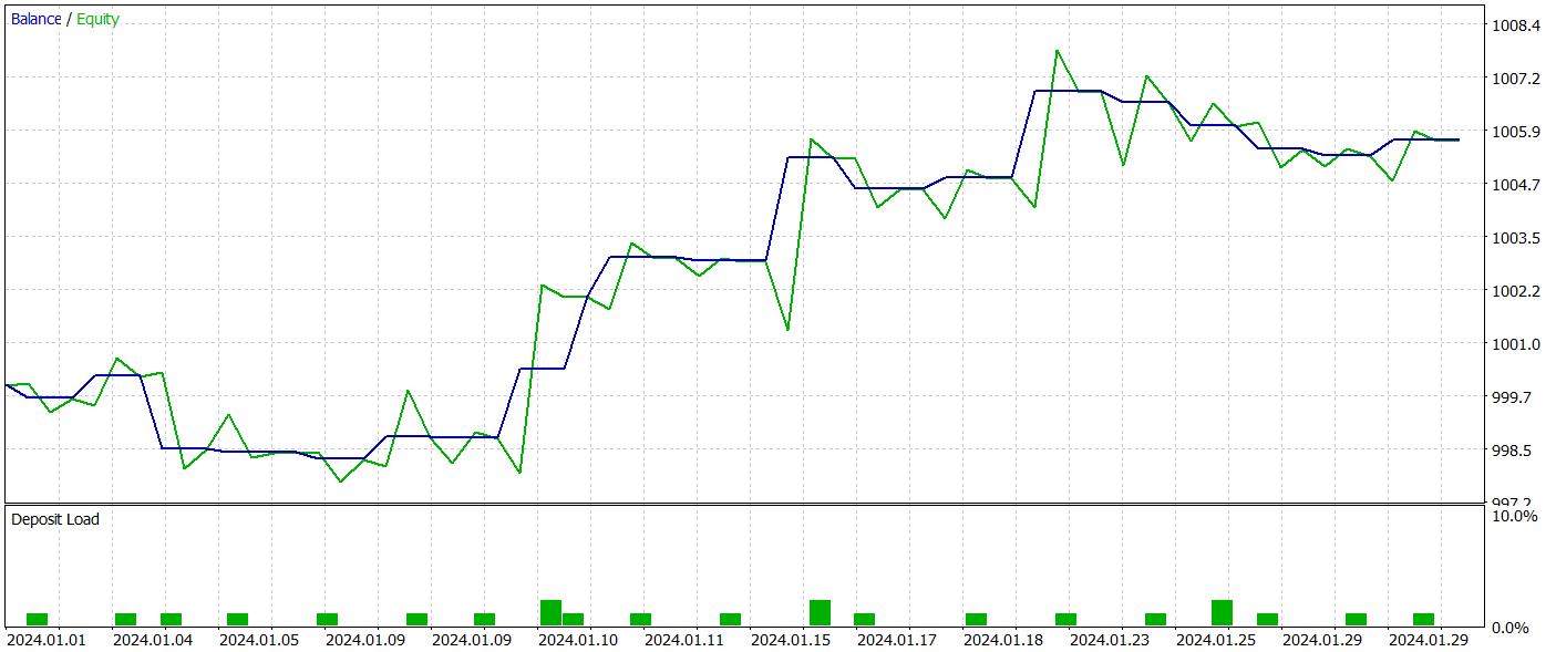
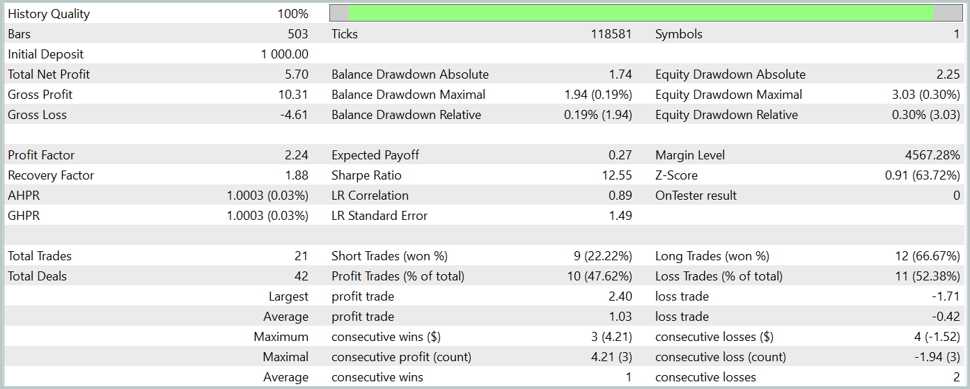
During the testing period, the trained model executed 21 trades, just over 47% of which were closed with a profit. It is worth noting that long positions showed significantly higher profitability (66% compared to 22%). Clearly, additional model training is required. Nevertheless, the average profitable trade was 2.5 times larger than the average loss-making one, allowing the model to achieve an overall profit during the test period.

In my subjective opinion, the model turned out to be rather heavy. This is likely due in large part to the use of scene-conditioned attention mechanisms. However, employing a similar approach in the HyperDet3D method generated better results with lower computational cost.

That said, the small number of trades and the short testing period in both cases do not allow us to draw any definitive conclusions about the long-term effectiveness of the method.

Conclusion

The SEFormer method is well-adapted for point cloud analysis and effectively captures local dependencies even in noisy conditions - a key factor for accurate forecasting. This opens up promising opportunities for more precise market movement predictions and improved decision-making strategies.

In the practical part of this article, we implemented our vision of the proposed approaches using MQL5. have trained and tested the model on real historical data. The results demonstrate the potential of the proposed method. However, before deploying the model in real trading scenarios, it is essential to train it over a longer historical period and conduct comprehensive testing of the trained policy.

References

• SEFormer: Structure Embedding Transformer for 3D Object Detection
• Other articles from this series

Programs used in the article

#	Issued to	Type	Description
1	Research.mq5	Expert Advisor	EA for collecting examples
2	ResearchRealORL.mq5	Expert Advisor	EA for collecting examples using the Real-ORL method
3	Study.mq5	Expert Advisor	Model training EA
4	Test.mq5	Expert Advisor	Model testing EA
5	Trajectory.mqh	Class library	System state description structure
6	NeuroNet.mqh	Class library	A library of classes for creating a neural network
7	NeuroNet.cl	Library	OpenCL program code library