
Neural Networks in Trading: Scene-Aware Object Detection (HyperDet3D)

Introduction
In recent years, object detection has garnered significant attention. Based on feature learning and volumetric convolution, PointNet++ emphasizes local geometry, elegantly analyzing raw point clouds. This has led to its widespread adoption as a backbone network in various object detection models.
However, the attributes of similar objects can be ambiguous, which degrades model performance. As a result, the model's applicability becomes limited, or its architecture must be made more complex. The authors of the paper "HyperDet3D: Learning a Scene-conditioned 3D Object Detector" observed that scene-level information provides prior knowledge that helps resolve ambiguity in object attribute interpretation. This, in turn, prevents illogical detection outcomes from a scene understanding perspective.
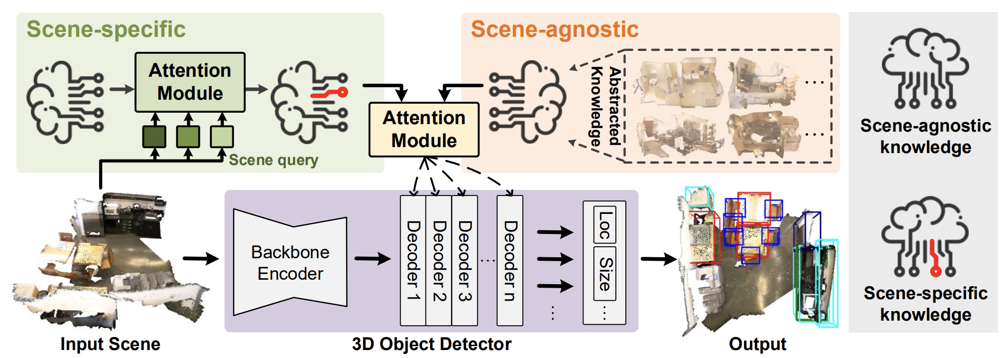
The paper introduces the HyperDet3D algorithm for 3D object detection in point clouds, which uses a hypernetwork-based architecture. HyperDet3D learns scene-conditioned information and incorporates scene-level knowledge into the network parameters. This allows the 3D object detector to dynamically adapt to varying input data. Specifically, scene-conditioned knowledge can be decomposed into two levels: scene-invariant information and scene-specific information.
To capture scene-invariant knowledge, the authors propose learning embeddings utilized by the hypernetwork and iteratively updated as the model is trained on diverse scenes. This scene-invariant information is typically abstracted from the characteristics of the training data and can be leveraged by the detector during inference.
Moreover, since conventional detectors maintain a fixed set of parameters when detecting objects across different scenes, the authors of HyperDet3D propose integrating scene-specific information to adapt the detector to a particular scene at inference time. This is achieved by analyzing how closely the current scene aligns with—or deviates from—the general representation, using the specific input as a query.
The paper introduces a novel module structure called Multi-head Scene-Conditioned Attention (MSA). MSA enables the aggregation of prior knowledge with candidate object features, thereby facilitating more effective object detection.
1. The HyperDet3D Algorithm
The HyperDet3D model includes three main components:
- A backbone Encoder
- An object Decoder layer
- A detection head
The input point cloud is first processed by the backbone, which downsamples the points to generate initial object candidates and coarsely extracts their features using hierarchical architectures. The authors propose using PointNet++ as the backbone network.
Next, the object decoder layers refine the candidate features, integrating scene-conditioned prior knowledge into the object-level representations. The detection head then regresses bounding boxes based on the locations and refined features of these candidate objects.
To enable HyperDet3D to be aware of scene-level meta-information, the authors introduce a HyperNetwork, which is a neural network used to parameterize the trainable parameters of the primary network. Unlike standard deep neural networks that maintain fixed parameters during inference, hypernetworks offer flexibility by adapting parameters based on the input data.
HyperDet3D applies a scene-conditioned hypernetwork to incorporate prior knowledge into the parameters of the Transformer decoder layers. This allows the detection network to dynamically adapt to varying input scenes. The key idea is to enrich the object representation 𝒐 formed from the candidate set generated by the backbone encoder, using prior knowledge parameterized by 𝑾 and provided by scene-conditioned hypernetworks.
The parameters generated by the scene-conditioned hypernetworks are divided into scene-invariant and scene-specific components.
To obtain scene-invariant knowledge, the authors propose training a set of n scene-agnostic embedding vectors 𝒁a, which are then consumed by the hypernetwork. The output of this hypernetwork is a weight matrix 𝑾a, which parameterizes the scene-invariant prior knowledge.
Since object properties are refined iteratively through a sequence of decoder layers, they can be progressively fused with the outputs of the scene-invariant hypernetwork. This network abstracts prior knowledge across diverse 3D scenes. As a result, HyperDet3D not only maintains generalized scene-conditioned knowledge across all decoder levels but also conserves computational resources by sharing knowledge through rich feature hierarchies.
To obtain scene-specific knowledge, the model learns a set of embeddings 𝒁s analogous to 𝒁a. But in this case, 𝒁s should capture information unique to individual scenes. This is achieved through a cross-attention block, where the embedding of the current scene is compared against the learned scene-specific embeddings 𝒁s. Through the attention mechanism, the model assesses how well 𝒁s aligns with the current scene (or how much it deviates) in the embedding space.
An official visualization of the HyperDet3D method is provided below.
2. Implementation in MQL5
After considering the theoretical aspects of the HyperDet3D method, we move on to the practical part of our article, in which we implement our vision of the proposed approaches.
Let us say up front: we have a significant amount of work ahead. To manage this efficiently, we will divide the implementation into several logical modules. So, let's roll up our sleeves and get started.
2.1 Scene-Specific Knowledge Module
We begin by building the module responsible for learning scene-specific knowledge. As discussed in the theoretical section, cross-attention is used to match the current scene with the scene-specific knowledge embeddings. Accordingly, we will define a new class, CNeuronSceneSpecific, as a subclass of the cross-attention block CNeuronMLCrossAttentionMLKV. The structure of the new class is shown below.
class CNeuronSceneSpecific :  public CNeuronMLCrossAttentionMLKV
  {
protected:
   CNeuronBaseOCL    cOne;
   CNeuronBaseOCL    cSceneSpecificKnowledge;
   //---
   virtual bool      feedForward(CNeuronBaseOCL *NeuronOCL) override;
   virtual bool      feedForward(CNeuronBaseOCL *NeuronOCL, CBufferFloat *Context) override
                                 { return feedForward(NeuronOCL); }
   //---
   virtual bool      calcInputGradients(CNeuronBaseOCL *NeuronOCL, CBufferFloat *SecondInput,
                                                                   CBufferFloat *SecondGradient,
                                                        ENUM_ACTIVATION SecondActivation = None) override
                                 { return calcInputGradients(NeuronOCL); }
   virtual bool      updateInputWeights(CNeuronBaseOCL *NeuronOCL, CBufferFloat *Context) override
                                 { return updateInputWeights(NeuronOCL); }
   virtual bool      calcInputGradients(CNeuronBaseOCL *NeuronOCL) override;
   virtual bool      updateInputWeights(CNeuronBaseOCL *NeuronOCL) override;

public:
                     CNeuronSceneSpecific(void) {};
                    ~CNeuronSceneSpecific(void) {};
   //---
   virtual bool      Init(uint numOutputs, uint myIndex, COpenCLMy *open_cl,
                          uint window, uint window_key, uint heads, uint heads_kv,
                          uint units_count, uint units_count_kv, uint layers, uint layers_to_one_kv,
                          ENUM_OPTIMIZATION optimization_type, uint batch);
   //---
   virtual int       Type(void) override  const   {  return defNeuronSceneSpecific;   }
   //---
   virtual bool      Save(int const file_handle) override;
   virtual bool      Load(int const file_handle) override;
   //---
   virtual bool      WeightsUpdate(CNeuronBaseOCL *source, float tau) override;
   virtual void      SetOpenCL(COpenCLMy *obj) override;
  };
Here, it is important to highlight one fundamental difference between our new class and its parent. The parent class requires two sources of data to function correctly: the input data and a context. In our new class, however, the context is represented by learned scene-specific data derived from the training set. This data is learned through two internal layers: cOne and cSceneSpecificKnowledge. Essentially, this forms a two-layer MLP that takes a scalar input (1) and generates a tensor representing scene-specific knowledge. As you might expect, during inference, this tensor remains static. However, during training, the model "writes" the necessary information into it.
Following this logic, we exclude pointers to the external context from the methods of our new class.
All objects are declared statically, allowing us to leave the class constructor and destructor "empty". Object initialization is performed in the Init method. In its parameters, we obtain the main constants of the object architecture. The functionality of the parameters used is similar to the relevant method of the parent class.
bool CNeuronSceneSpecific::Init(uint numOutputs, uint myIndex, COpenCLMy *open_cl,
                                uint window, uint window_key, uint heads, uint heads_kv,
                                uint units_count, uint units_count_kv, uint layers, uint layers_to_one_kv,
                                ENUM_OPTIMIZATION optimization_type, uint batch)
  {
   if(!CNeuronMLCrossAttentionMLKV::Init(numOutputs, myIndex, open_cl, window, window_key, heads, 16, heads_kv,
                              units_count, units_count_kv, layers, layers_to_one_kv, optimization_type, batch))
      return false;
In the body of the method, we first call the initialization method of the parent class, passing along all the parameters received. This parent method handles parameter validation and the setup of inherited components.
Next, we initialize the previously mentioned scene-specific MLP.
Note that the first layer contains only a single constant input. The second layer generates a set of embedding vectors representing scene-specific knowledge. Each embedding vector is 16 elements in length. The number of embeddings is defined by method parameters and depends on the complexity of the environment being modeled.
   if(!cOne.Init(16 * units_count_kv, 0, OpenCL, 1, optimization, iBatch))
      return false;
   CBufferFloat *out = cOne.getOutput();
   if(!out.BufferInit(1, 1) || !out.BufferWrite())
      return false;
   if(!cSceneSpecificKnowledge.Init(0, 1, OpenCL, 16 * units_count_kv, optimization, iBatch))
      return false;
//---
   return true;
  }
Before concluding the method, we return a boolean value indicating the success or failure of the initialization to the calling function.
The initialization method of our new class is relatively short and concise. For good reason: the core functionality has already been implemented in the parent class. This pattern holds true not only for the initialization method. This also applies to the feedForward method, whose parameters include a pointer to the source input data.
bool CNeuronSceneSpecific::feedForward(CNeuronBaseOCL *NeuronOCL)
  {
   if(bTrain && !cSceneSpecificKnowledge.FeedForward(cOne.AsObject()))
      return false;
In the body of the method, we first need to generate a matrix of learned context-dependent representations of the scene. But we perform this operation only in the model training process, when the resulting tensor is changed as we adjust the parameters of our MLP. During the model operation, these learned values are static and do not need to be recomputed. We simply reuse the pre-saved information.
Finally, we call the feedForward method of the parent class, passing in our scene-specific knowledge tensor as the context input.
   if(!CNeuronMLCrossAttentionMLKV::feedForward(NeuronOCL, cSceneSpecificKnowledge.getOutput()))
      return false;
//---
   return true;
  }
The backpropagation pass methods are constructed in a similar way. For the sake of conciseness and to keep the article from growing excessively long, I suggest studying them independently. The full implementation of the class and all its methods can be found in the attached materials.
2.2 Constructing the MSA Block
Now, we move on to constructing the Multi-Head Scene-Conditioned Attention (MSA) block. Naturally, we will inherit the core functionality from one of the previously implemented attention blocks. The structure of the new class CNeuronMLMHSceneConditionAttention is presented below.
class CNeuronMLMHSceneConditionAttention  :  public CNeuronMLMHAttentionMLKV
  {
protected:
   CLayer            cSceneAgnostic;
   CLayer            cSceneSpecific;
   //---
   virtual bool      feedForward(CNeuronBaseOCL *NeuronOCL) override;
   //---
   virtual bool      calcInputGradients(CNeuronBaseOCL *prevLayer) override;
   virtual bool      updateInputWeights(CNeuronBaseOCL *NeuronOCL) override;

public:
                     CNeuronMLMHSceneConditionAttention(void) {};
                    ~CNeuronMLMHSceneConditionAttention(void) {};
   //---
   virtual bool      Init(uint numOutputs, uint myIndex, COpenCLMy *open_cl,
                          uint window, uint window_key, uint heads, uint heads_kv,
                          uint units_count, uint layers, uint layers_to_one_kv,
                          ENUM_OPTIMIZATION optimization_type, uint batch) override;
   //---
   virtual int       Type(void) override  const   {  return defNeuronMLMHSceneConditionAttention;   }
   //---
   virtual bool      Save(int const file_handle) override;
   virtual bool      Load(int const file_handle) override;
   //---
   virtual bool      WeightsUpdate(CNeuronBaseOCL *source, float tau) override;
   virtual void      SetOpenCL(COpenCLMy *obj) override;
  };
Within this structure, you'll notice the declaration of two new objects of type CLayer. One will store context-dependent representations of the scene, while the other holds general object-related information that is independent of the scene.
It is important to note that the presence of these two objects does not restrict the creation of deeper, nested neural layers for object identification. In this case, the CLayer objects are used as dynamic arrays. While the number of internal neural layers is defined by the user during object initialization.
All internal objects are declared as static, allowing us to leave the constructor and destructor empty. As usual, the initialization of all internal and inherited objects is performed in the Init method.
bool CNeuronMLMHSceneConditionAttention::Init(uint numOutputs, uint myIndex, COpenCLMy *open_cl,
                                              uint window, uint window_key, uint heads, uint heads_kv,
                                              uint units_count, uint layers, uint layers_to_one_kv,
                                              ENUM_OPTIMIZATION optimization_type, uint batch)
  {
   if(!CNeuronBaseOCL::Init(numOutputs, myIndex, open_cl, window * units_count, optimization_type, batch))
      return false;
In the method parameters we receive the main constants that determine the architecture of the created object. And in the body of the method, we immediately call the relevant ancestor method. However, in this case we use the method not of the direct parent class, but of the base fully connected layer CNeuronBaseOCL. This is due to significant differences in the structure and size of inherited objects.
After the operations of the ancestor initialization method have successfully completed, we will save the architectural constants of our new class.
   iWindow = fmax(window, 1);
   iWindowKey = fmax(window_key, 1);
   iUnits = fmax(units_count, 1);
   iHeads = fmax(heads, 1);
   iLayers = fmax(layers, 1);
   iHeadsKV = fmax(heads_kv, 1);
   iLayersToOneKV = fmax(layers_to_one_kv, 1);
Then we calculate the dimensions of the internal objects.
   uint num_q = iWindowKey * iHeads * iUnits;               //Size of Q tensor
   uint num_kv = 2 * iWindowKey * iHeadsKV * iUnits;        //Size of KV tensor
   uint q_weights = (iWindow * iHeads) * iWindowKey;        //Size of weights' matrix of Q tenzor
   uint kv_weights = 2 * (iWindow * iHeadsKV) * iWindowKey; //Size of weights' matrix of KV tenzor
   uint scores = iUnits * iUnits * iHeads;                  //Size of Score tensor
   uint mh_out = iWindowKey * iHeads * iUnits;              //Size of multi-heads self-attention
   uint out = iWindow * iUnits;                             //Size of out tensore
   uint w0 = (iWindowKey * iHeads + 1) * iWindow;           //Size W0 tensor
   uint ff_1 = 4 * (iWindow + 1) * iWindow;                 //Size of weights' matrix 1-st feed forward layer
   uint ff_2 = (4 * iWindow + 1) * iWindow;                 //Size of weights' matrix 2-nd feed forward layer
WE add 2 more local variables for temporary storage of pointers to neural layer objects.
   CNeuronBaseOCL *base = NULL;
   CNeuronSceneSpecific *ss = NULL;
This concludes the preparatory work. Next, we organize a loop with the number of iterations equal to the number of internal layers specified in the method parameters by the user. At each iteration of this loop, we create objects of one inner layer. Accordingly, after the full completion of the specified number of loop iterations, we create a complete set of objects necessary for the normal functioning of the required number of internal neural layers.
   for(uint i = 0; i < iLayers; i++)
     {
      CBufferFloat *temp = NULL;
      for(int d = 0; d < 2; d++)
        {
         //--- Initilize Q tensor
         temp = new CBufferFloat();
         if(CheckPointer(temp) == POINTER_INVALID)
            return false;
         if(!temp.BufferInit(num_q, 0))
            return false;
         if(!temp.BufferCreate(OpenCL))
            return false;
         if(!QKV_Tensors.Add(temp))
            return false;
In the body of the loop, we immediately create another nested loop of 2 iterations. In the body of the nested loop, we save data buffers to record the main flow data of the forward pass and the corresponding error gradients of the backpropagation pass. This 2-iteration loop allows us to create a mirror architecture for the feed-forward and backpropagation passes.
Here first we create a buffer to record the generated Query entities. Then we create a buffer for recording the weight matrix for generating this entity.
         //--- Initilize Q weights
         temp = new CBufferFloat();
         if(CheckPointer(temp) == POINTER_INVALID)
            return false;
         if(!temp.BufferInit(q_weights, 0))
            return false;
         if(!temp.BufferCreate(OpenCL))
            return false;
         if(!QKV_Weights.Add(temp))
            return false;
Note that previously we always filled the weight matrix with random values that were adjusted during the model training process. This time, we have created a buffer with zero values. This is due to the implementation of the hypernetwork architecture, which will generate this matrix taking into account the analyzed scene.
We repeat similar operations to generate Key and Value entity data buffers. But here we also add the ability to use one tensor for several internal layers. Therefore, before creating data buffers, we check the feasibility of such operations.
         if(i % iLayersToOneKV == 0)
           {
            //--- Initilize KV tensor
            temp = new CBufferFloat();
            if(CheckPointer(temp) == POINTER_INVALID)
               return false;
            if(!temp.BufferInit(num_kv, 0))
               return false;
            if(!temp.BufferCreate(OpenCL))
               return false;
            if(!KV_Tensors.Add(temp))
               return false;
            //--- Initilize KV weights
            temp = new CBufferFloat();
            if(CheckPointer(temp) == POINTER_INVALID)
               return false;
            if(!temp.BufferInit(kv_weights, 0))
               return false;
            if(!temp.BufferCreate(OpenCL))
               return false;
            if(!KV_Weights.Add(temp))
               return false;
           }
Next, we add a buffer to store the dependency coefficients.
         //--- Initialize scores
         temp = new CBufferFloat();
         if(CheckPointer(temp) == POINTER_INVALID)
            return false;
         if(!temp.BufferInit(scores, 0))
            return false;
         if(!temp.BufferCreate(OpenCL))
            return false;
         if(!S_Tensors.Add(temp))
            return false;
And another buffer to store the results of multi-headed attention.
         //--- Initialize multi-heads attention out
         temp = new CBufferFloat();
         if(CheckPointer(temp) == POINTER_INVALID)
            return false;
         if(!temp.BufferInit(mh_out, 0))
            return false;
         if(!temp.BufferCreate(OpenCL))
            return false;
         if(!AO_Tensors.Add(temp))
            return false;
As before, the results of multi-headed attention will scale to the size of the original data. We will write the result of this operation into the corresponding data buffer.
         //--- Initialize attention out
         temp = new CBufferFloat();
         if(CheckPointer(temp) == POINTER_INVALID)
            return false;
         if(!temp.BufferInit(out, 0))
            return false;
         if(!temp.BufferCreate(OpenCL))
            return false;
         if(!FF_Tensors.Add(temp))
            return false;
Let;'s also add FeedForward block operation buffers.
         //--- Initialize Feed Forward 1
         temp = new CBufferFloat();
         if(CheckPointer(temp) == POINTER_INVALID)
            return false;
         if(!temp.BufferInit(4 * out, 0))
            return false;
         if(!temp.BufferCreate(OpenCL))
            return false;
         if(!FF_Tensors.Add(temp))
            return false;
         //--- Initialize Feed Forward 2
         if(i == iLayers - 1)
           {
            if(!FF_Tensors.Add(d == 0 ? Output : Gradient))
               return false;
            continue;
           }
         temp = new CBufferFloat();
         if(CheckPointer(temp) == POINTER_INVALID)
            return false;
         if(!temp.BufferInit(out, 0))
            return false;
         if(!temp.BufferCreate(OpenCL))
            return false;
         if(!FF_Tensors.Add(temp))
            return false;
        }
As in the parent's corresponding method, we do not create new output buffers for the final internal layer of the FeedForward block. Instead, we point directly to the buffers inherited from the base fully connected layer. These buffers are used for inter-layer data exchange. And we write to them directly during execution, avoiding unnecessary data transfer between internal and external interfaces.
After initializing data buffers for the feed-forward and backpropagation data streams, we proceed to initialize the weight matrices. However, in our case, the generation of the Query, Key, and Value entities, adapted to the current scene state, relies on two hypernetworks: one for scene-independent (prior) knowledge of objects and one for scene-dependent (contextual) knowledge. These hypernetworks also require initialization.
At this point, different implementation strategies are possible. As you know, Key and Value, unlike Query, may not need to be generated at every internal layer. Therefore, we allocate them into a separate tensor. We could, theoretically, create separate hypernetworks for each corresponding weight matrix. However, that approach is suboptimal in terms of performance. Because it would increase the number of sequential operations. Instead, we opted to generate the required tensors in parallel using unified hypermodels, and then distribute the outputs into the appropriate data buffers.
However, Key and Value are not required on every internal layer. Therefore, we take that into account and, in such cases, simply utilize a model that returns a smaller result tensor.
Sounds logical? Great—let’s move on to implementation. First, we divide the operation stream into two branches, depending on whether or not Key-Value tensors need to be generated. The execution algorithm is identical for both streams. The only difference lies in the size of the resulting tensors.
      if(i % iLayersToOneKV == 0)
        {
         //--- Initilize Scene-Specific layers
         ss = new CNeuronSceneSpecific();
         if(!ss)
            return false;
         if(!ss.Init((q_weights + kv_weights), cSceneSpecific.Total(), OpenCL, iWindow, iWindowKey,
                                                     4, 2, iUnits, 100, 2, 2, optimization, iBatch))
            return false;
         if(!cSceneSpecific.Add(ss))
            return false;
First, we work with the context-dependent representation model. Here, we create and initialize a dynamic instance of the scene-specific knowledge module that we implemented earlier. A pointer to this newly created object is stored in the cSceneSpecific array,which forms part of the context-conditioned model.
However, one key nuance should be noted here. The scene-specific knowledge module was built upon a cross-attention block, which takes as input the analyzed state of the scene. And it returns a tensor of the appropriate dimensions, enriched with context-dependent knowledge. The issue is that the size of the input tensor may not match the required dimensions of the target weight matrix. To resolve this, we introduce a fully connected scaling layer that adjusts the dimensions accordingly.
         base = new CNeuronBaseOCL();
         if(!base)
            return false;
         if(!base.Init(0, cSceneSpecific.Total(), OpenCL, (q_weights + kv_weights), optimization, iBatch))
            return false;
         base.SetActivationFunction(TANH);
         if(!cSceneSpecific.Add(base))
            return false;
This scaling layer employs the hyperbolic tangent (tanh) as its activation function, which outputs values in the range [-1, 1]. As a result, the context-conditioned knowledge about the scene essentially acts as a flagging mechanism, indicating the likelihood or presence of certain objects within the analyzed scene.
For the scene-independent prior knowledge model, we use a two-layer MLP, similar in structure to the one described earlier for maintaining context-conditioned embeddings.
         //--- Initilize Scene-Agnostic layers
         base = new CNeuronBaseOCL();
         if(!base)
            return false;
         if(!base.Init((q_weights + kv_weights), cSceneAgnostic.Total(), OpenCL, 1, optimization, iBatch))
            return false;
         temp = base.getOutput();
         if(!temp.BufferInit(1, 1) || !temp.BufferWrite())
            return false;
         if(!cSceneAgnostic.Add(base))
            return false;
         base = new CNeuronBaseOCL();
         if(!base)
            return false;
         if(!base.Init(0, cSceneAgnostic.Total(), OpenCL, (q_weights + kv_weights), optimization, iBatch))
            return false;
         if(!cSceneAgnostic.Add(base))
            return false;
        }
If there is no need to generate a Key-Value tensor, we create similar objects, but smaller in size.
      else
        {
         //--- Initilize Scene-Specific layers
         ss = new CNeuronSceneSpecific();
         if(!ss)
            return false;
         if(!ss.Init(q_weights, cSceneSpecific.Total(), OpenCL, iWindow, iWindowKey,
                                           4, 2, iUnits, 100, 2, 2, optimization, iBatch))
            return false;
         if(!cSceneSpecific.Add(ss))
            return false;
         base = new CNeuronBaseOCL();
         if(!base)
            return false;
         if(!base.Init(0, cSceneSpecific.Total(), OpenCL, q_weights, optimization, iBatch))
            return false;
         base.SetActivationFunction(TANH);
         if(!cSceneSpecific.Add(base))
            return false;
         //--- Initilize Scene-Agnostic layers
         base = new CNeuronBaseOCL();
         if(!base)
            return false;
         if(!base.Init(q_weights, cSceneAgnostic.Total(), OpenCL, 1, optimization, iBatch))
            return false;
         temp = base.getOutput();
         if(!temp.BufferInit(1, 1) || !temp.BufferWrite())
            return false;
         if(!cSceneAgnostic.Add(base))
            return false;
         base = new CNeuronBaseOCL();
         if(!base)
            return false;
         if(!base.Init(0, cSceneAgnostic.Total(), OpenCL, q_weights, optimization, iBatch))
            return false;
         if(!cSceneAgnostic.Add(base))
            return false;
        }
For the multi-head attention result data scaling layer and the FeedForward block, we use regular matrices of training parameters initialized with random parameters.
      //--- Initilize Weights0
      temp = new CBufferFloat();
      if(CheckPointer(temp) == POINTER_INVALID)
         return false;
      if(!temp.Reserve(w0))
         return false;
      float k = (float)(1 / sqrt(iWindow + 1));
      for(uint w = 0; w < w0; w++)
        {
         if(!temp.Add(GenerateWeight() * 2 * k - k))
            return false;
        }
      if(!temp.BufferCreate(OpenCL))
         return false;
      if(!FF_Weights.Add(temp))
         return false;
      //--- Initilize FF Weights
      temp = new CBufferFloat();
      if(CheckPointer(temp) == POINTER_INVALID)
         return false;
      if(!temp.Reserve(ff_1))
         return false;
      for(uint w = 0; w < ff_1; w++)
        {
         if(!temp.Add(GenerateWeight() * 2 * k - k))
            return false;
        }
      if(!temp.BufferCreate(OpenCL))
         return false;
      if(!FF_Weights.Add(temp))
         return false;
      //---
      temp = new CBufferFloat();
      if(CheckPointer(temp) == POINTER_INVALID)
         return false;
      if(!temp.Reserve(ff_2))
         return false;
      k = (float)(1 / sqrt(4 * iWindow + 1));
      for(uint w = 0; w < ff_2; w++)
        {
         if(!temp.Add(GenerateWeight() * 2 * k - k))
            return false;
        }
      if(!temp.BufferCreate(OpenCL))
         return false;
      if(!FF_Weights.Add(temp))
         return false;
We also add moment buffers that we use in the process of optimizing the created matrices of training parameters. The number of moment buffers is determined by the specified parameter optimization method.
      //---
      for(int d = 0; d < (optimization == SGD ? 1 : 2); d++)
        {
         temp = new CBufferFloat();
         if(CheckPointer(temp) == POINTER_INVALID)
            return false;
         if(!temp.BufferInit((d == 0 || optimization == ADAM ? w0 : iWindow), 0))
            return false;
         if(!temp.BufferCreate(OpenCL))
            return false;
         if(!FF_Weights.Add(temp))
            return false;
         //--- Initilize FF Weights
         temp = new CBufferFloat();
         if(CheckPointer(temp) == POINTER_INVALID)
            return false;
         if(!temp.BufferInit((d == 0 || optimization == ADAM ? ff_1 : 4 * iWindow), 0))
            return false;
         if(!temp.BufferCreate(OpenCL))
            return false;
         if(!FF_Weights.Add(temp))
            return false;
         temp = new CBufferFloat();
         if(CheckPointer(temp) == POINTER_INVALID)
            return false;
         if(!temp.BufferInit((d == 0 || optimization == ADAM ? ff_2 : iWindow), 0))
            return false;
         if(!temp.BufferCreate(OpenCL))
            return false;
         if(!FF_Weights.Add(temp))
            return false;
        }
     }
After successfully initializing all the specified objects, we move on to the next iteration of the loop, in which we will create similar objects for the subsequent inner layer.
At the end of the initialization method, we initialize the auxiliary buffer for storing temporary data and return the logical result of the operations to the calling program.
   if(!Temp.BufferInit(MathMax((num_q + num_kv)*iWindow, out), 0))
      return false;
   if(!Temp.BufferCreate(OpenCL))
      return false;
//---
   SetOpenCL(OpenCL);
//---
   return true;
  }
The complex structure and large number of objects make it difficult to understand the algorithm being constructed. Moreover, we need to carefully monitor the flow of information and data transfer between objects during the implementation of feed-forward and backpropagation pass methods. And we will start with the construction of the feedForward method.
bool CNeuronMLMHSceneConditionAttention::feedForward(CNeuronBaseOCL *NeuronOCL)
  {
   CNeuronBaseOCL *ss = NULL, *sa = NULL;
   CBufferFloat *q_weights = NULL, *kv_weights = NULL, *q = NULL, *kv = NULL;
In the method parameters, we receive a pointer to the source data object. However, we do not organize a check of the relevance of the received index. Because we do not plan to directly access the source data object at this stage. However, we will do a little preparatory work, during which we will create local variables for temporary storage of pointers to various objects. And then we'll create a loop to iterate through the internal layers of our block.
   for(uint i = 0; i < iLayers; i++)
     {
      //--- Scene-Specific
      ss = cSceneSpecific[i * 2];
      if(!ss.FeedForward(NeuronOCL))
         return false;
      ss = cSceneSpecific[i * 2 + 1];
      if(!ss.FeedForward(cSceneSpecific[i * 2]))
         return false;
Inside the loop, we begin by generating the weight coefficients required to construct the Query, Key, and Value entities, using the previously defined hypernetworks.
First, based on the scene state description received from the calling program, we generate the matrix of context-dependent parameters. As described earlier, after enriching this tensor with context-specific knowledge, we rescale it to match the dimensions of the required parameter matrix.
At the same time, we generate the matrix of scene-independent parameters.
      //--- Scene-Agnostic
      sa = cSceneAgnostic[i * 2 + 1];
      if(bTrain && !sa.FeedForward(cSceneAgnostic[i * 2]))
         return false;
Note that the scene-independent parameter matrix is only generated during model training. During operation, the matrix remains static. So there is no need to regenerate it for each feed-forward pass.
Next, we perform element-wise multiplication of the two matrices. The result is the final weight matrix, which we then distribute into the previously initialized data buffers. It's important to note that this is a single generated weight matrix, which is split into two parts. One part is used to create Query entities. The second part is used for Key and Value entities. However, Key and Value are not necessarily formed on every layer. Therefore, we need to branch the operation flow depending on whether the Key-Value tensor generation is required.
Before doing so, we carry out a bit of preliminary setup. Specifically, we transfer a pointer to the input data object of the current internal layer into a local variable.
CBufferFloat *inputs = (i == 0 ? NeuronOCL.getOutput() : FF_Tensors.At(6 * i - 4));
Here we store the pointer to the internal layer's input. This means that the pointer received from the external program is only passed into the first internal layer. For all subsequent layers, we use the outputs from the previous internal layer.
We also store in local variables the pointers to the data buffers of the weight parameters and the Query tensor, both of which are used regardless of which of the two processing paths we follow.
      q_weights = QKV_Weights[i * 2];
      q = QKV_Tensors[i * 2];
If it is necessary to form a Key-Value tensor, we first perform element-wise multiplication of the two weight matrices formed above. And we write the result of the operation into the temporary data storage buffer.
      if(i % iLayersToOneKV == 0)
        {
         if(IsStopped() || !ElementMult(ss.getOutput(), sa.getOutput(), GetPointer(Temp)))
            return false;
We save pointers to the weight and Key-Value entity value buffers in local variables.
         kv_weights = KV_Weights[(i / iLayersToOneKV) * 2];
         kv = KV_Tensors[(i / iLayersToOneKV) * 2];
Then we distribute the common tensor of weight parameters across two data buffers.
         if(IsStopped() || !DeConcat(q_weights, kv_weights, GetPointer(Temp), iHeads, 2 * iHeadsKV,
                                                                              iWindow * iWindowKey))
            return false;
         if(IsStopped() || !MatMul(inputs, kv_weights, kv, iUnits, iWindow, 2 * iHeadsKV * iWindowKey, 1))
            return false;
        }
After that we will form a tensor of Key-Value entities by matrix multiplication of the initial data tensor of the current internal layer by the obtained matrix of weight coefficients.
If there is no need to form a Key-Value entity tensor, we only perform the operation of element-wise multiplication of two parameter matrices with the results written to the corresponding data buffer. Bevause in this case, our hypernetworks form only a weight matrix of the Query entity.
      else
        {
         if(IsStopped() || !ElementMult(ss.getOutput(), sa.getOutput(), q_weights))
            return false;
        }
The formation of the Query entity value tensor is performed in any case. Therefore, we implement this operation in the general flow.
      if(IsStopped() || !MatMul(inputs, q_weights, q, iUnits, iWindow, iHeads * iWindowKey, 1))
         return false;
At this stage, the implementation of hypernetworks into the attention algorithm is completed. Then follows the mechanism that is already familiar to us: Self-Attention. First, we determine the results of multi-headed attention.
      //--- Score calculation and Multi-heads attention calculation
      CBufferFloat *temp = S_Tensors[i * 2];
      CBufferFloat *out = AO_Tensors[i * 2];
      if(IsStopped() || !AttentionOut(q, kv, temp, out))
         return false;
Then we reduce the dimensionality of the resulting output tensor.
      //--- Attention out calculation
      temp = FF_Tensors[i * 6];
      if(IsStopped() ||
         !ConvolutionForward(FF_Weights[i * (optimization == SGD ? 6 : 9)], out, temp,
                                                   iWindowKey * iHeads, iWindow, None))
         return false;
After that we sum up the results of the Self-Attention block with the original data and normalize the resulting tensor.
      //--- Sum and normilize attention
      if(IsStopped() || !SumAndNormilize(temp, inputs, temp, iWindow, true))
         return false;
Next the data passes through the FeedForward block.
      //--- Feed Forward
      inputs = temp;
      temp = FF_Tensors[i * 6 + 1];
      if(IsStopped() ||
         !ConvolutionForward(FF_Weights[i * (optimization == SGD ? 6 : 9) + 1], inputs, temp,
                                                                 iWindow, 4 * iWindow, LReLU))
         return false;
      out = FF_Tensors[i * 6 + 2];
      if(IsStopped() ||
         !ConvolutionForward(FF_Weights[i * (optimization == SGD ? 6 : 9) + 2], temp, out,
                                                           4 * iWindow, iWindow, activation))
         return false;
Then we sum and normalize the data.
      //--- Sum and normilize out
      if(IsStopped() || !SumAndNormilize(out, inputs, out, iWindow, true))
         return false;
     }
//--- result
   return true;
  }
We repeat the operations for all internal layers. After we complete all loop iterations, the logical result of executing the method operations is returned to the calling program .
I hope at this stage, you understand how our class's algorithm works. But there is another nuance related to the distribution of the error gradient during the backpropagation pass - its algorithm is implemented in the calcInputGradients method.
bool CNeuronMLMHSceneConditionAttention::calcInputGradients(CNeuronBaseOCL *prevLayer)
  {
   if(CheckPointer(prevLayer) == POINTER_INVALID)
      return false;
In the method parameters, as usual, we receive a pointer to the object of the previous layer, to which we must propagate the error gradient in accordance with the influence of the original data on the final result. In the body of the method, we immediately check the relevance of the received pointer. After that, we create several local variables for temporary storage of pointers to objects.
   CBufferFloat *out_grad = Gradient;
   CBufferFloat *kv_g = KV_Tensors[KV_Tensors.Total() - 1];
   CNeuronBaseOCL *ss = NULL, *sa = NULL;
Then we organize a reverse loop through the internal layers.
   for(int i = int(iLayers - 1); (i >= 0 && !IsStopped()); i--)
     {
      if(i == int(iLayers - 1) || (i + 1) % iLayersToOneKV == 0)
         kv_g = KV_Tensors[(i / iLayersToOneKV) * 2 + 1];
As you are aware, the gradient backpropagation algorithm mirrors the feed-forward pass, with all operations executed in reverse order. For this reason, we structured a reverse iteration loop over the internal layers of our block.
Let me remind you that the second half of the forward pass operations directly replicated the corresponding logic in the parent class. Consequently, we begin the first half of our gradient backpropagation method by reusing the corresponding method from the parent class.
We start by backpropagating the error gradient through the FeedForward block.
      //--- Passing gradient through feed forward layers
      if(IsStopped() ||
        !ConvolutionInputGradients(FF_Weights[i * (optimization == SGD ? 6 : 9) + 2], out_grad,
                       FF_Tensors[i * 6 + 1], FF_Tensors[i * 6 + 4], 4 * iWindow, iWindow, None))
         return false;
      CBufferFloat *temp = FF_Tensors[i * 6 + 3];
      if(IsStopped() ||
        !ConvolutionInputGradients(FF_Weights[i * (optimization == SGD ? 6 : 9) + 1],
                     FF_Tensors[i * 6 + 4], FF_Tensors[i * 6], temp, iWindow, 4 * iWindow, LReLU))
         return false;
After that we sum the error gradient from the two information streams.
      //--- Sum and normilize gradients
      if(IsStopped() || !SumAndNormilize(out_grad, temp, temp, iWindow, false))
         return false;
And then we propagate the error gradient through the Multi-Head Self-Attention block.
      //--- Sum and normilize gradients
      if(IsStopped() || !SumAndNormilize(out_grad, temp, temp, iWindow, false))
         return false;
      out_grad = temp;
      //--- Split gradient to multi-heads
      if(IsStopped() ||
        !ConvolutionInputGradients(FF_Weights[i * (optimization == SGD ? 6 : 9)], out_grad,
                AO_Tensors[i * 2], AO_Tensors[i * 2 + 1], iWindowKey * iHeads, iWindow, None))
         return false;
      //--- Passing gradient to query, key and value
      sa = cSceneAgnostic[i * 2 + 1];
      ss = cSceneSpecific[i * 2 + 1];
      if(i == int(iLayers - 1) || (i + 1) % iLayersToOneKV == 0)
        {
         if(IsStopped() ||
         !AttentionInsideGradients(QKV_Tensors[i * 2], QKV_Tensors[i * 2 + 1],
                 KV_Tensors[(i / iLayersToOneKV) * 2], kv_g, S_Tensors[i * 2], AO_Tensors[i * 2 + 1]))
            return false;
        }
      else
        {
         if(IsStopped() ||
           !AttentionInsideGradients(QKV_Tensors[i * 2], QKV_Tensors[i * 2 + 1],
             KV_Tensors[i / iLayersToOneKV * 2], GetPointer(Temp), S_Tensors[i * 2], AO_Tensors[i * 2 + 1]))
            return false;
         if(IsStopped() ||
           !SumAndNormilize(kv_g, GetPointer(Temp), kv_g, iWindowKey, false, 0, 0, 0, 1))
            return false;
        }
Here, special attention should be paid to how the error gradient is propagated to the Key-Value tensor. The nuance lies in collecting error gradients from all internal layers influenced by a given tensor. A more detailed explanation of this algorithm is provided in the article dedicated to the parent class.
We then proceed to backpropagate the error gradient to the level of the input data along the main information flow.
      CBufferFloat *inp = NULL;
      if(i == 0)
        {
         inp = prevLayer.getOutput();
         temp = prevLayer.getGradient();
        }
      else
        {
         temp = FF_Tensors.At(i * 6 - 1);
         inp = FF_Tensors.At(i * 6 - 4);
        }
      if(IsStopped() ||
        !MatMulGrad(inp, temp, QKV_Weights[i * 2], QKV_Weights[i * 2 + 1], QKV_Tensors[i * 2 + 1],
                                                          iUnits, iWindow, iHeads * iWindowKey, 1))
         return false;
      //--- Sum and normilize gradients
      if(IsStopped() || !SumAndNormilize(out_grad, temp, temp, iWindow, false, 0, 0, 0, 1))
         return false;
We also propagate the error gradient to the hypernetworks in accordance with their influence on the overall result of the model.
      //---
      if((i % iLayersToOneKV) == 0)
        {
         if(IsStopped() ||
           !MatMulGrad(inp, GetPointer(Temp), KV_Weights[i / iLayersToOneKV * 2],
                       KV_Weights[i / iLayersToOneKV * 2 + 1], KV_Tensors[i / iLayersToOneKV * 2 + 1],
                                                        iUnits, iWindow, 2 * iHeadsKV * iWindowKey, 1))
            return false;
         if(IsStopped() || !SumAndNormilize(GetPointer(Temp), temp, temp, iWindow, false, 0, 0, 0, 1))
            return false;
         if(!Concat(QKV_Weights[i * 2 + 1], KV_Weights[i / iLayersToOneKV * 2 + 1], ss.getGradient(),
                                                           iHeads, 2 * iHeadsKV, iWindow * iWindowKey))
            return false;
         if(!ElementMultGrad(ss.getOutput(), ss.getGradient(), sa.getOutput(), sa.getGradient(),
                                                   ss.getGradient(), ss.Activation(), sa.Activation()))
            return false;
        }
      else
        {
         if(!ElementMultGrad(ss.getOutput(), ss.getGradient(), sa.getOutput(), sa.getGradient(),
                                              QKV_Weights[i * 2 + 1], ss.Activation(), sa.Activation()))
            return false;
        }
      if(i > 0)
         out_grad = temp;
     }
After this, we move to the next iteration of our loop through internal layers.
It is important to note that in the main operation loop, we only propagated the error gradient down to the hypernetworks, but we did not propagate it through them. This introduces a couple of nuances. First, our scene-independent hypernetwork consists of only two layers. The first is static, always outputting a constant value of 1. And the second contains trainable parameters and returns the actual result. In the main operations stream, we pass the error gradient only to the second layer. Propagating the gradient to the static first layer would be meaningless. Of course, this is a specific case. If the hypermodel had more layers, we would need to implement gradient backpropagation logic for all layers containing trainable parameters.
The second nuance pertains to the scene-dependent hypernetwork. In this implementation, all parameters are generated based on the scene description received from the calling program. As a result, the entire error gradient must be propagated to that level. To maintain the integrity of the main data flow, we chose to handle gradient propagation for this model in a separate loop. Again, this is a specific implementation choice. If we were to derive the scene description from a different source (e.g., the output of a preceding internal layer), we would need to propagate the gradient accordingly.
Let's return to the algorithm of our gradient backpropagation method. After completing the reverse iteration over internal layers, we store in the gradient buffer of the previous layer the results representing how the input data influenced the model's output through the main data flow. We must now add the contribution from the hypernetworks to this buffer. To do this, we first store a pointer to the gradient buffer of the previous layer in a local variable. Then, we temporarily assign a pointer to our auxiliary data buffer to the current layer object.
   CBufferFloat *inp_grad = prevLayer.getGradient();
   if(!prevLayer.SetGradient(GetPointer(Temp), false))
      return false;
Now we can propagate the error gradient down to the previous layer without fear of losing previously saved data. We create a loop iterating over the objects of our context-dependent hypernetwork; in its body we propagate the error gradient to the level of the source data layer. At each iteration, we add the current result to the previously accumulated gradient.
   for(int i = int(iLayers - 2); (i >= 0 && !IsStopped()); i -= 2)
     {
      ss = cSceneSpecific[i];
      if(IsStopped() || !ss.calcHiddenGradients(cSceneSpecific[i + 1]))
         return false;
      if(IsStopped() || !prevLayer.calcHiddenGradients(ss, NULL))
         return false;
      if(IsStopped() ||
        !SumAndNormilize(prevLayer.getGradient(), inp_grad, inp_grad, iWindow, false, 0, 0, 0, 1))
         return false;
     }
After the successful execution of the loop operations, we return to the object of the previous layer a pointer to its buffer with the already accumulated error gradient from all information flows.
   if(!prevLayer.SetGradient(inp_grad, false))
      return false;
//---
   return true;
  }
The error gradient is distributed in full and we return to the calling program the logical result of executing the operations of our error gradient distribution method. I suggest you familiarize yourself with the method of updating the model parameters independently. You can find the full code of this class and all its methods in the attachment.
2.3 Constructing the Complete HyperDet3D Algorithm
Earlier, we built the individual components of the HyperDet3D algorithm. Now it's time to bring everything together into a single, cohesive structure. And while this may seem relatively straightforward, there are a few important nuances worth highlighting.
For this experiment, I chose to base the integration on the Pointformer architecture discussed in the previous article. The key modification here is the replacement of the global attention block with our newly constructed MSA module. This operation is quite simple. Especially since we've left all method parameters unchanged, including the class initialization method. However, there's a catch: all objects within the original CNeuronPointFormer class were declared as static. As a result, we cannot inherit from the class and modify the types of its internal objects directly. Therefore, we create a duplicate of the class, in which we adjust the types of the necessary internal objects to incorporate the new functionality. The structure of the new class is shown below.
class CNeuronHyperDet   :  public CNeuronPointNet2OCL
  {
protected:
   CNeuronMLMHSparseAttention    caLocalAttention[2];
   CNeuronMLCrossAttentionMLKV   caLocalGlobalAttention[2];
   CNeuronMLMHSceneConditionAttention  caGlobalAttention[2];
   CNeuronLearnabledPE           caLocalPE[2];
   CNeuronLearnabledPE           caGlobalPE[2];
   CNeuronBaseOCL                cConcatenate;
   CNeuronConvOCL                cScale;
   //---
   CBufferFloat                  *cbTemp;
   //---
   virtual bool      feedForward(CNeuronBaseOCL *NeuronOCL) override ;
   //---
   virtual bool      calcInputGradients(CNeuronBaseOCL *NeuronOCL) override;
   virtual bool      updateInputWeights(CNeuronBaseOCL *NeuronOCL) override;

public:
                     CNeuronHyperDet(void) {};
                    ~CNeuronHyperDet(void) { delete cbTemp; }
   //---
   virtual bool      Init(uint numOutputs, uint myIndex, COpenCLMy *open_cl,
                          uint window, uint units_count, uint output, bool use_tnets,
                          ENUM_OPTIMIZATION optimization_type, uint batch) override;
   //---
   virtual int       Type(void) override   const   {  return defNeuronHyperDet; }
   //---
   virtual bool      Save(int const file_handle) override;
   virtual bool      Load(int const file_handle) override;
   //---
   virtual bool      WeightsUpdate(CNeuronBaseOCL *source, float tau) override;
   virtual void      SetOpenCL(COpenCLMy *obj) override;
  };
We will not delve into the methods of this class, as all of them were created by directly copying the corresponding methods from the CNeuronPointFormer class.
The model architecture, along with all interaction and training scripts, were also borrowed from the previous article. Therefore, we will not discuss them now. The complete source code for all programs used in the preparation of this article is available in the attachment.
3. Testing
We have conducted extensive work to implement our own interpretation of the approaches proposed by the authors of the HyperDet3D method. Now it's time to move on to the final part of our article. Here, we train and test the models that incorporate the described techniques.
As always, to train the models we use real historical data of the EURUSD instrument, with the H1 timeframe, for the whole of 2023. All indicator parameters were set to their default values. The training process itself follows the exact algorithm outlined in the previous article. So we will focus only on the results of testing the trained Actor policy, which are presented below.
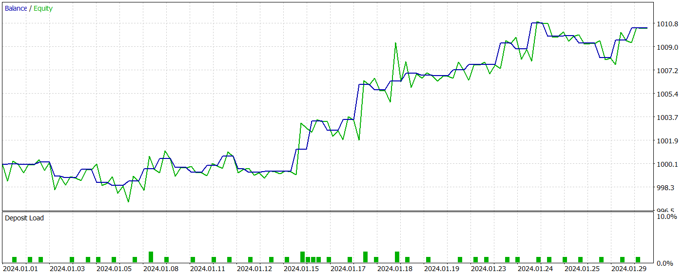
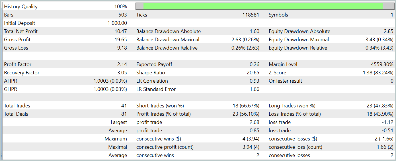
The trained model was tested on historical data from January 2024, which was not part of the training dataset. During this period, the model executed 41 trades, with 56% of them closing in profit. Notably, the largest winning trade was 2.4 times larger than the largest loss, and the average profitable trade exceeded the average losing trade by 67%. These outcomes resulted in a profit factor of 2.14 and a Sharpe ratio of 20.65.
Overall, the model achieved a 1% profit during the test period, while the maximum drawdown on equity did not exceed 0.34%. The balance drawdown was even lower. The equity curve shows a steady balance increase, and the account exposure remained within 1–2%.
The general impression of the results is positive. The model shows promise. However, the short testing period and limited number of trades prevent us from making conclusions about the model's long-term stability. Before it can be used in live trading, further training on a larger historical dataset and more comprehensive testing will be required.
Conclusion
In this article, we explored the HyperDet3D method, which integrates scene-conditioned hypernetworks into a Transformer architecture to embed prior knowledge. This allows the model to adapt effectively to different scenes in object detection tasks by dynamically tuning detector parameters based on scene information. This makes the system more universal and powerful.
In the practical section, we implemented our interpretation of the proposed concepts using MQL5, integrating them into our custom model architecture. The test results demonstrate the potential of the model. However, further work is needed before it can be applied in real-world financial markets.
References
Programs used in the article
| # | Issued to | Type | Description |
|---|---|---|---|
| 1 | Research.mq5 | Expert Advisor | EA for collecting examples |
| 2 | ResearchRealORL.mq5 | Expert Advisor | EA for collecting examples using the Real-ORL method |
| 3 | Study.mq5 | Expert Advisor | Model training EA |
| 4 | Test.mq5 | Expert Advisor | Model testing EA |
| 5 | Trajectory.mqh | Class library | System state description structure |
| 6 | NeuroNet.mqh | Class library | A library of classes for creating a neural network |
| 7 | NeuroNet.cl | Library | OpenCL program code library |
Translated from Russian by MetaQuotes Ltd.
Original article: https://www.mql5.com/ru/articles/15859
Warning: All rights to these materials are reserved by MetaQuotes Ltd. Copying or reprinting of these materials in whole or in part is prohibited.
This article was written by a user of the site and reflects their personal views. MetaQuotes Ltd is not responsible for the accuracy of the information presented, nor for any consequences resulting from the use of the solutions, strategies or recommendations described.

 Building a Custom Market Regime Detection System in MQL5 (Part 1): Indicator
- Free trading apps
- Over 8,000 signals for copying
- Economic news for exploring financial markets
You agree to website policy and terms of use