ONNX統合の課題を克服する

MetaTrader 5 — トレーディングシステム | 31 5月 2024, 15:48

724

Omega J Msigwa

はじめに

ONNX (Open Neural Network Exchange)は、洗練されたAIベースのMQL5プログラムを作成する方法に革命をもたらします。MetaTrader 5のこの新しいテクノロジーは、機械学習への前進であり、その目的には他にはない多くの可能性を示しています。ただし、ONNXにはいくつかの課題があり、それを解決する手がかりが全くない場合、頭痛の種になる可能性があります。

フィードフォワードニューラルネットワークのような単純なAI技術を導入する場合は、導入プロセスにそれほど問題はないかもしれませんが、実世界でのプロジェクトはもっと複雑なものが多いため、時系列データの抽出、ビッグデータの前処理や次元を減らすための変換など、多くのことをおこなう必要があるかもしれません。また、1つの大規模プロジェクトで複数のモデルを使用する必要がある場合、ONNXの展開が複雑になる可能性があります。

ONNXは、AIモデルのみを保存する機能を備えた自己完結型のツールです。訓練済みのモデルを反対側で実行するために必要なものがすべて同梱されているわけではありません。最終的なONNXモデルをどのように展開するかは、ユーザーが決める必要があります。この記事では、データのスケーリングと正規化、モデルへの次元削減の導入、時系列予測のためのONNXモデルの導入という3つの課題について説明します。

この記事は、読者が機械学習とAI理論の基本的な知識を持っていて、少なくとも1度か2度MQL5でONNXモデルを使用してみたことがあることを前提としています。

データ前処理の課題を克服する

機械学習の文脈では、データ処理とは、データセットの特徴量の値を特定の範囲に変換するプロセスを指します。この変換は、機械学習モデルのために、より一貫性のあるデータ表現を達成することを目的としています。スケーリングのプロセスは、いくつかの理由から非常に重要です。

機械学習モデルのパフォーマンスを向上させる：多くの機械学習アルゴリズム、特にK近傍法(KNN)やサポートベクトルマシン(SVM)のような距離ベースのものは、データ点間の距離計算に依存しています。特徴量のスケールが大きく異なる場合（例えば、ある特徴量は千分の一、別の特徴量は十分の一）、スケールの大きい特徴量が距離計算を支配することになり、パフォーマンスが最適化されません。スケーリングは、すべての特徴量を同じような範囲に置き、モデルがデータポイント間の実際の関係に集中できるようにします。

訓練の収束を早める：勾配降下ベースの最適化アルゴリズムは、ニューラルネットワークやその他のモデルで一般的に使用され、損失関数の勾配に基づいて最適解に向かってステップを踏みます。特徴量のスケールが異なると、勾配の大きさも大きく異なり、オプティマイザが効率的に最小値を求めることが難しくなります。スケーリングは、勾配の範囲をより一定にし、収束を早めるのに役立ちます。

数値演算の安定性を確保：機械学習アルゴリズムの中には、スケールが大きく異なる特徴量では計算が不安定になるものがあります。スケーリングは、このような数値的な問題を防ぎ、モデルが正確に計算を実行できるようにするのに役立ちます。

一般的なスケーリング技法

正規化(MinMaxScaling)：この技法は、特定の範囲（多くの場合、0～1または-1～1）に特徴量をスケーリングします。
標準化（Zスコア正規化）：この技法は、各特徴量から平均を引くことでデータをセンタリングし、それを標準偏差で割ることでスケーリングします。

この正規化のプロセスは非常に重要なのですが、ネット上ではその正しい方法を説明しているものは多くありません。学習データに使用したのと同じスケーリング技法とそのパラメータを、テストデータにもモデルを展開する際にも適用しなければなりません。

同じスケーラーのアナロジー：訓練データに「収入」を表す特徴量があるとします。スケーラーは、訓練中に所得の最小値と最大値（標準化の場合は平均値と標準偏差）を学習します。テストデータに別のスケーラーを使用すると、訓練時に見た範囲外の所得値に遭遇する可能性があります。これは予期せぬスケーリングにつながり、訓練データとテストデータの間に矛盾をもたらす可能性があります。

スケーラーのアナロジーに同じパラメータを使用します。高さを測る定規を想像してみてください。訓練用とテスト用で異なる単位（インチとセンチ）が記された定規を使えば、測定値は比較できません。同様に、訓練データとテストデータで異なるスケーラーを使用すると、訓練中に学習したモデルの参照枠が崩れます。

要するに、同じスケーラーを使用することで、訓練中もテスト中もモデルが一貫してデータを見ることができ、より信頼性が高く解釈しやすい結果につながります。

Scikit-learn.preprocessing Pythonモジュールからスケーリング技法を使用することができます。ONNXモデルをビルドし、同じPython言語で展開している限り、すべて問題ありません。

from sklearn.preprocessing import MinMaxScaler, StandardScaler
import numpy as np

# Example data
data = np.array([[1000, 2], [500, 1], [2000, 4], [800, 3]])

# Create a MinMaxScaler object
scaler_minmax = MinMaxScaler()

# Fit the scaler on the training data (learn min/max values)
scaler_minmax.fit(data)

# Transform the data using the fitted scaler
data_scaled_minmax = scaler_minmax.transform(data)

print("Original data:\n", data)
print("\nMin Max Scaled data:\n", data_scaled_minmax)

しかし、学習させたモデルをMQL5言語で使用するとすると、状況は難しくなります。Pythonでは、様々な方法でスケーラーを保存することができますが、Pythonにはオブジェクトを格納する独自の方法があり、他のプログラミング言語よりも処理が簡単なため、Metaエディタでスケーラーを抽出するのは難しくなります。一番良いのは、MQL5でデータを前処理し、スケーラーを保存して、CSVファイルにスケーリングされたデータを保存し、Pythonコードを使用して読み込むことでしょう。

以下は、データの前処理のロードマップです。

市場からデータを収集し、スケーリングする
スケーラーを保存する
スケーリングしたデータをCSVファイルに保存する

01：市場からのデータ収集とスケーリング

1000本の日足の始値、高値、安値、終値のレートを収集します。パターン認識問題を作成して、価格が始値より上で引けた場合は強気、そうでない場合は弱気のシグナルを割り当てます。このパターンでLSTM AIモデルを訓練することで、何がこのパターンに寄与しているのかを理解させ、一旦十分に訓練されれば取引シグナルを提供できるようにしようとしているのです。

ONNXのデータ収集スクリプト内で、以下をおこないます。

まずは、必要なライブラリを含めることから始めます。

#include <MALE5\preprocessing.mqh> //This library contains the normalization techniques for machine learning
#include <MALE5\MatrixExtend.mqh>

StandardizationScaler scaler; //We want to use z-normalization/standardization technique for this project

次に、価格情報を収集する必要があります。

input int data_size = 10000; //number of bars to collect for our dataset

MqlRates rates[];
//+------------------------------------------------------------------+
//| Script program start function                                    |
//+------------------------------------------------------------------+
void OnStart()
  {
//--- vector.CopyRates is lacking we are going to copy rates in normal way

   ArraySetAsSeries(rates, true);    
   if (CopyRates(Symbol(), PERIOD_D1, 1, data_size, rates)<-1)
     {
       printf("Failed to collect data Err=%d",GetLastError());
       return;
     }
   

   matrix OHLC(data_size, 4);
   for (int i=0; i<data_size; i++) //Get OHLC values and save them to a matrix
     {
       OHLC[i][0] = rates[i].open;
       OHLC[i][1] = rates[i].high;
       OHLC[i][2] = rates[i].low;
       
        if (rates[i].close>rates[i].open)
          OHLC[i][3] = 1; //Buy signal
        else if (rates[i].close<rates[i].open)
          OHLC[i][3] = 0; //sell signal
     }

//---
  }

思い出してください。スケーリングは独立変数に対しておこなうので、列をスケーリングできるx行列を得るために、データ行列をそれぞれx行列とy行列とベクトルに分割します。

   matrix x;
   vector y;
   MatrixExtend::XandYSplitMatrices(OHLC, x, y);  //WE split the data into x and y | The last column in the matrix will be assigned to the y vector 
     
//--- Standardize the data
   
   x = scaler.fit_transform(x);

02：スケーラーの保存

先に述べたように、後で使用するためにスケーラーを保存しておく必要があります。

   if (!scaler.save(Symbol()+"-SCALER"))
      return;

このコードスニペットを実行すると、バイナリファイルの入ったフォルダが作成されます。この2つのファイルには、標準化スケーラー用のパラメータが含まれています。このパラメータを使用して、保存したスケーラーインスタンスを読み込む方法は後で説明します。

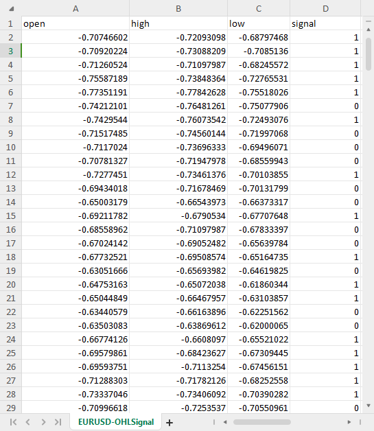
03：スケーリングしたデータをCSVファイルに保存する

最後に、後でPythonコードで使用できるように、スケーリングしたデータをCSVファイルに保存する必要があります。

   OHLC = MatrixExtend::concatenate(x, y); //We apped the y column to the scaled x matrix, this is the opposite of XandYsplitMatrices function
   if (!MatrixExtend::WriteCsv(Symbol()+"-OHLSignal.csv",OHLC,"open,high,low,signal",false,8))       
    {
     DebugBreak();
     return;
    }

結果

時系列データの課題を克服する

GRU、LSTM、RNNのような時系列ディープラーニングモデルが他のモデルと比較して株式市場の予測に優れていることを示唆する研究はいくつかあります。一定期間にわたるパターンを理解する能力があるため、私を含め、データサイエンスコミュニティのほとんどのアルゴリズムトレーダーは、これらの特定のモデルに合わせています。

これらのモデルを使った時系列予測に適したデータを準備するために、追加で書かなければならないコードがいくつかあることがわかりました。

時系列モデルを扱ったことがある人なら、おそらくこれと似たような関数やコードを見たことがあるでしょう。

def get_sequential_data(data, time_step):
    if dataset.empty is True:
      print("Failed to create sequences from an empty dataset")
      return

    Y = data.iloc[:, -1].to_numpy() # get the last column from the dataset and assign it to y numpy 1D array
    X = data.iloc[:, :-1].to_numpy() # Get all the columns from data array except the last column, assign them to x numpy 2D array

    X_reshaped = []
    Y_reshaped = []

    for i in range(len(Y) - time_step + 1):
        X_reshaped.append(X[i:i + time_step])
        Y_reshaped.append(Y[i + time_step - 1])

    return np.array(X_reshaped), np.array(Y_reshaped)

この関数は、LSTMのような時系列モデルにとって非常に重要であり、データ準備をおこないます。

データを一定サイズ(time_step)のシーケンスに分割する
特徴量（過去の情報）とターゲット（予測値）を分離する
データをLSTMモデルに適した形式に整形する

このデータ準備は、LSTMモデルに構造化された方法で最も関連性の高い情報を提供するのに役立ち、学習の高速化、メモリ管理の改善、予測精度の向上につながる可能性があります。

LSTMはシーケンスを扱うことができますが、リアルタイムのデータは連続的な情報の流れをもたらします。それでもなお、予測をおこなう際にモデルが考慮する過去のデータの時間窓を定義する必要があります。そのため、この関数は訓練やテストだけでなく、リアルタイムの予測にも必要となります。y配列は必要ありませんが、x配列の形を変えるコードは必要です。MetaTrader 5ではリアルタイムの予測をおこなうため、これと同じような関数をMQL5で作成する必要があります。

その前に、get_sequential_data関数が時間ステップ値が7のときに返すxとyのNumpy配列の次元を確認してみましょう。

X_reshaped, Y_reshaped = get_sequential_data(dataset, step_size)

print(f"x_shape{X_reshaped.shape} y_shape{Y_reshaped.shape}")

出力

x_shape(9994, 7, 3) y_shape(9994,)

返されるx配列は3次元配列、言い換えればテンソル、返されるyデータは1次元行列、言い換えればベクトルです。MQL5で同様の関数を作成する際には、この点を考慮する必要があります。

では、CTSDataProcessorという名前の簡単なクラスを作ってみましょう。

class CTSDataProcessor 
  {
CTensors *tensor_memory[]; //Tensor objects may be hard to track in memory once we return them from a function, this keeps track of them
bool xandysplit;

public:
                     CTSDataProcessor (void);
                    ~CTSDataProcessor (void);
                    
                     CTensors *extract_timeseries_data(const matrix<double> &x, const int time_step); //for real time predictions
                     CTensors *extract_timeseries_data(const matrix<double> &MATRIX, vector &y, const int time_step); //for training and testing purposes 
  };

似たような名前の2つの関数extract_timeseries_dataは、一方がyベクトルを返さないことを除けば、同じような働きをします。

CTSDataProcessor ::CTSDataProcessor (void)
 {
   xandysplit = true; //by default obtain the y vector also
 }
//+------------------------------------------------------------------+
//|                                                                  |
//+------------------------------------------------------------------+
CTensors *CTSDataProcessor ::extract_timeseries_data(const matrix<double> &x,const int time_step)
 {
  CTensors *timeseries_tensor;
  timeseries_tensor = new CTensors(0);
  ArrayResize(tensor_memory, 1);
  tensor_memory[0] = timeseries_tensor;
  
  xandysplit = false; //In this function we do not obtain the y vector
  
  vector y;
  timeseries_tensor = extract_timeseries_data(x, y, time_step);
  
  xandysplit = true; //restore the original condition
   
  return timeseries_tensor;
 }
//+------------------------------------------------------------------+
//|                                                                  |
//+------------------------------------------------------------------+
CTensors *CTSDataProcessor ::extract_timeseries_data(const matrix &MATRIX, vector &y,const int time_step)
 {
  CTensors *timeseries_tensor;
  timeseries_tensor = new CTensors(0);
  ArrayResize(tensor_memory, 1);
  tensor_memory[0] = timeseries_tensor;
  
  matrix<double> time_series_data = {};
  matrix x = {}; //store the x variables converted to timeseries
  vector y_original = {};
  y.Init(0);
  
  if (xandysplit) //if we are required to obtain the y vector also split the given matrix into x and y
     if (!MatrixExtend::XandYSplitMatrices(MATRIX, x, y_original))
       {
         printf("%s failed to split the x and y matrices in order to make a tensor",__FUNCTION__);
         return timeseries_tensor;
       }
  
  x = xandysplit ? x : MATRIX; 
  
  for (ulong sample=0; sample<x.Rows(); sample++) //Go throught all the samples
    {
      matrix<double> time_series_matrix = {};
      vector<double> timeseries_y(1);
      
      for (ulong time_step_index=0; time_step_index<(ulong)time_step; time_step_index++)
        {
            if (sample + time_step_index >= x.Rows())
                break;
             
             time_series_matrix = MatrixExtend::concatenate(time_series_matrix, x.Row(sample+time_step_index), 0);
             
             if (xandysplit)
               timeseries_y[0] = y_original[sample+time_step_index]; //The last value in the column is assumed to be a y value so it gets added to the y vector
        }
      
      if (time_series_matrix.Rows()<(ulong)time_step)
        continue;
        
        timeseries_tensor.Append(time_series_matrix);
         
        if (xandysplit)
         y = MatrixExtend::concatenate(y, timeseries_y);
    }
   
   return timeseries_tensor;
 }

では、ONNX challenges EAというEAの中で、これらの関数を使用して時系列データを抽出してみましょう。

#include <Timeseries Deep Learning\tsdataprocessor.mqh>

input int time_step_ = 7;
//it is very important the time step value matches the one used during training in  a python script


CTSDataProcessor ts_dataprocessor;
CTensors *ts_data_tensor;
//+------------------------------------------------------------------+
//| Expert initialization function                                   |
//+------------------------------------------------------------------+
int OnInit()
  {
//---
   
   if (!onnx.Init(lstm_model))
     return INIT_FAILED;
     
   string headers;  
   matrix data = MatrixExtend::ReadCsv("EURUSD-OHLSignal.csv",headers); //let us open the same data so that we don't get confused along the way
   
   matrix x;
   vector y;
      
   ts_data_tensor = ts_dataprocessor.extract_timeseries_data(data, y, time_step_);
   
   printf("x_shape %s y_shape (%d,)",ts_data_tensor.shape(),y.Size());
 }

出力

GD      0       07:21:14.710    ONNX challenges EA (EURUSD,H1)  Warning: CTensors::shape assumes all matrices in the tensor have the same size
IG      0       07:21:14.710    ONNX challenges EA (EURUSD,H1)  x_shape (9994, 7, 3) y_shape (9994,)

Pythonのコードと同じ次元が得られました。

ONNXの目的は、ある言語で構築された機械学習モデルを、他の言語でも同じように機能させることです。つまり、Pythonでモデルを構築し、それを実行した場合、そのモデルが提供する精度と正確さは、他の言語（この場合はMQL5言語）でも、同じデータを変換せずに使用した場合とほぼ同じになるはずです。

この場合、ONNXモデルをMQL5で使用する前に、両プラットフォームの同じデータでモデルをテストし、同じ精度が得られるかどうか確認する必要があります。このモデルを検証してみましょう。

入力層に10ニューロン、隠れ層に1ニューロンのLSTMモデルを作成し、Adamオプティマイザを学習の進捗に割り当てました。

from keras.optimizers import Adam
from keras.callbacks import EarlyStopping

learning_rate = 1e-3
patience = 5 #if this number of epochs validation loss is unchanged stop the process


model = Sequential()

model.add(LSTM(units=10, input_shape=(step_size, dataset.shape[1]-1))) #Input layer
model.add(Dense(units=10, activation='relu', kernel_initializer='he_uniform'))
model.add(Dropout(0.3))
model.add(Dense(units=len(classes_in_data), activation = 'softmax')) #last layer outputs = classes in data

model.compile(optimizer=Adam(learning_rate=learning_rate), loss="binary_crossentropy", metrics=['accuracy'])

出力

Model: "sequential"
_________________________________________________________________
 Layer (type)                Output Shape              Param #   
=================================================================
 lstm (LSTM)                 (None, 10)                560       
                                                                 
 dense (Dense)               (None, 10)                110       
                                                                 
 dropout (Dropout)           (None, 10)                0         
                                                                 
 dense_1 (Dense)             (None, 2)                 22        
                                                                 
=================================================================
Total params: 692 (2.70 KB)
Trainable params: 692 (2.70 KB)
Non-trainable params: 0 (0.00 Byte)
_________________________________________________________________

patienceを5エポックに設定し、batch_size = 64で100エポック訓練しました。

from keras.utils import to_categorical

y_train = to_categorical(y_train, num_classes=len(classes_in_data)) #ONE-HOT encoding
y_test = to_categorical(y_test, num_classes=len(classes_in_data)) #ONE-HOT encoding

early_stopping = EarlyStopping(monitor='val_loss', patience = patience, restore_best_weights=True)

history = model.fit(x_train, y_train, epochs = 100 , validation_data = (x_test,y_test), callbacks=[early_stopping], batch_size=64, verbose=2)

LSTMモデルは77回目のエポックで収束し、損失は0.3000、精度スコアは0.8876になりました。

Epoch 75/100
110/110 - 1s - loss: 0.3076 - accuracy: 0.8856 - val_loss: 0.2702 - val_accuracy: 0.8983 - 628ms/epoch - 6ms/step
Epoch 76/100
110/110 - 1s - loss: 0.2968 - accuracy: 0.8856 - val_loss: 0.2611 - val_accuracy: 0.9060 - 651ms/epoch - 6ms/step
Epoch 77/100
110/110 - 1s - loss: 0.3000 - accuracy: 0.8876 - val_loss: 0.2634 - val_accuracy: 0.9063 - 714ms/epoch - 6ms/step

損失と反復のグラフ

最後に、データセット全体でモデルをテストしました。

X_reshaped, Y_reshaped = get_sequential_data(dataset, step_size)

predictions = model.predict(X_reshaped)

predictions = classes_in_data[np.argmax(predictions, axis=1)]  # Find class with highest probability | converting predicted probabilities to classes

from sklearn.metrics import accuracy_score

print("LSTM model accuracy: ", accuracy_score(Y_reshaped, predictions))

以下がその結果です。

313/313 [==============================] - 2s 3ms/step

LSTM model accuracy:  0.9179507704622774

MQL5でONNXに保存されたこのLSTMモデルを使用する場合は、この精度値またはそれに近い値を期待する必要があります。

inp_model_nameはmodel.eurusd.D1.onnxでした。

output_path = inp_model_name
onnx_model = tf2onnx.convert.from_keras(model, output_path=output_path)
print(f"saved model to {output_path}")

このモデルをEAに組み込んでみましょう。

#include <Timeseries Deep Learning\onnx.mqh>
#include <Timeseries Deep Learning\tsdataprocessor.mqh>
#include <MALE5\metrics.mqh>

#resource "\\Files\\model.eurusd.D1.onnx" as uchar lstm_model[]

input int time_step_ = 7;
//it is very important the time step value matches the one used during training in  a python script

CONNX onnx;
CTSDataProcessor ts_dataprocessor;
CTensors *ts_data_tensor;

ライブラリonnx.mqhの中には、ONNXモデルを初期化し、予測をおこなう関数を持つONNXクラスしかありません。

class CONNX
  {
protected:

   bool initialized;
   long onnx_handle;
   void PrintTypeInfo(const long num,const string layer,const OnnxTypeInfo& type_info);
   long inputs[], outputs[];
   
   void replace(long &arr[]) { for (uint i=0; i<arr.Size(); i++) if (arr[i] <= -1) arr[i] = UNDEFINED_REPLACE; }
   string ConvertTime(double seconds);
   
public:
                     CONNX(void);
                    ~CONNX(void);
                     
                     bool Init(const uchar &onnx_buff[], ulong flags=ONNX_DEFAULT); //Initislized ONNX model from a resource uchar array with default flag
                     bool Init(string onnx_filename, uint flags=ONNX_DEFAULT); //Initializes the ONNX model from a .onnx filename given

                     virtual int predict_bin(const matrix &x, const vector &classes_in_data); //Returns the predictions for the current given matrix, this function is for real-time prediction
                     virtual vector predict_bin(CTensors &timeseries_tensor, const vector &classes_in_data); //gives out the vector for all the predictions | useful function for testing only
                     virtual vector predict_proba(const matrix &x); //Gives out the predictions for the current given matrix | this function is for realtime predictions
  };

最後に、ONNX challenges EAで、読み込んだLSTMモデルを実行しました。

int OnInit()
  {
   if (!onnx.Init(lstm_model))
     return INIT_FAILED;
     
   string headers;  
   matrix data = MatrixExtend::ReadCsv("EURUSD-OHLSignal.csv",headers); //let us open the same data so that we don't get confused along the way
   
   matrix x;
   vector y;
      
   ts_data_tensor = ts_dataprocessor.extract_timeseries_data(data, y, time_step_);
      
   vector classes_in_data = MatrixExtend::Unique(y); //Get the classes in the data
      
   vector preds = onnx.predict_bin(ts_data_tensor, classes_in_data);
   
   Print("LSTM Model Accuracy: ",Metrics::accuracy_score(y, preds));
   
//---
   return(INIT_SUCCEEDED);
  }

以下がその結果です。

2024.04.14 07:44:16.667 ONNX challenges EA (EURUSD,H1)  LSTM Model Accuracy: 0.9179507704622774

素晴らしいことに、Pythonのコードで得たのと同じ精度（有効数字）の値が得られましたた。これは、私たちのやり方がすべて正しかったことを物語っています。

では、このモデルを使用してリアルタイムの予測を立ててから先に進みましょう。

ONNX challenges REALTIME EAの内は次のようになります。

これまでテスト用に正規化されたデータを含むCSVファイルを使用していたのとは異なり、今回はリアルタイムデータセットで予測をおこなうため、ONNX形式のLSTMモデルにデータを供給する前に、一度保存したスケーラーを読み込んで毎回新しいデータに適用する必要があります。

#resource "\\Files\\model.eurusd.D1.onnx" as uchar lstm_model[]
#resource "\\Files\\EURUSD-SCALER\\mean.bin" as double standardization_scaler_mean[];
#resource "\\Files\\EURUSD-SCALER\\std.bin" as double standardization_scaler_std[];

ONNXモデルをリソースとして読み込んだ直後に、保存した平均値と標準値のバイナリファイルをインクルードする必要があります。

今回は、保存されたスケーラー値でインスタンス化するため、ポインタを用いて標準化スケーラーを呼び出します。

#include <Timeseries Deep Learning\onnx.mqh>
#include <Timeseries Deep Learning\tsdataprocessor.mqh>
#include <MALE5\preprocessing.mqh>

#resource "\\Files\\model.eurusd.D1.onnx" as uchar lstm_model[]
#resource "\\Files\\EURUSD-SCALER\\mean.bin" as double standardization_scaler_mean[];
#resource "\\Files\\EURUSD-SCALER\\std.bin" as double standardization_scaler_std[];

input int time_step_ = 7;
//it is very important the time step value matches the one used during training in  a python script

CONNX onnx;
StandardizationScaler *scaler;
CTSDataProcessor ts_dataprocessor;
CTensors *ts_data_tensor;

MqlRates rates[];
vector classes_ = {0,1};
//+------------------------------------------------------------------+
//| Expert initialization function                                   |
//+------------------------------------------------------------------+
int OnInit()
  {
//---
   
   if (!onnx.Init(lstm_model))
     return INIT_FAILED;
   
   scaler = new StandardizationScaler(standardization_scaler_mean, standardization_scaler_std); //laoding the saved scaler
   
//---
   return(INIT_SUCCEEDED);
  }

ここでは、すべての新しい入力データを正規化する方法を説明します。

void OnTick()
  { 
   if (CopyRates(Symbol(), PERIOD_D1, 1, time_step_, rates)<-1)
     {
       printf("Failed to collect data Err=%d",GetLastError());
       return;
     }
   
   matrix data(time_step_, 3);
   for (int i=0; i<time_step_; i++) //Get the independent values and save them to a matrix
     {
       data[i][0] = rates[i].open;
       data[i][1] = rates[i].high;
       data[i][2] = rates[i].low;
     }
   
   ts_data_tensor = ts_dataprocessor.extract_timeseries_data(data, time_step_);  //process the new data into timeseries 
   
   data = ts_data_tensor.Get(0); //This tensor contains only one matrix for the recent latest bars thats why we find it at the index 0
   data = scaler.transform(data); //Transform the new data 
   
   int signal = onnx.predict_bin(data, classes_);
   
   Comment("LSTM trade signal: ",signal);
  }

最後に、ストラテジーテスターでEAを実行しましたが、エラーはなく、予測はチャート上に正常に表示されました。

次元削減の課題を克服する

先に述べたように、機械学習モデルを使った実世界の問題解決では、タスクを達成するためにAIモデルコード以上のものが必要です。データ科学者が通常道具箱に持ち歩く便利な道具の1つに、PCA、LDA、NMF、Truncated SVDなどの次元削減アルゴリズムがあります。欠点はあるものの、次元削減アルゴリズムには以下のような利点もあります。

次元削減の利点

モデル性能の向上：高次元のデータは、特徴量空間が膨大なためにモデルが効果的に学習できないという、「次元の呪い」につながる可能性があります。PCAは複雑さを軽減し、分類、回帰、クラスタリングを含む様々な機械学習アルゴリズムの性能を向上させることができます。

より迅速な訓練と処理：高次元データに対する機械学習モデルの訓練には、計算コストがかかります。PCAは特徴量の数を減らすので、訓練時間が短縮され、必要な計算資源が少なくなる可能性があります。

過剰適合の削減：高次元は、モデルが学習データを記憶するが未知のデータに対してうまく汎化できないという、過剰適合のリスクを増大させる可能性があります。PCAは、最も情報量の多い特徴量に焦点を当てることで、このリスクを軽減するのに役立ちます。

スケーリング技法と同じように、Scikit-Learnが提供する主成分分析(PCA)のような次元削減技法を使えば良いですが、構築したものすべてに基づいて取引を含むほとんどの作業がおこなわれるMQL5で、このPCAを使用する方法を見つけるのは大変でしょう。

ONNXのデータ収集スクリプト内にPCAを追加しなければなりません。

#include <MALE5\Dimensionality Reduction\PCA.mqh>

CPCA *pca;

正規化処理がおこなわれる前に、x変数を正規化するためにPCA技法を追加します。

   MatrixExtend::XandYSplitMatrices(OHLC, x, y);  //WE split the data into x and y | The last column in the matrix will be assigned to the y vector 

//--- Reduce data dimension

   pca = new CPCA(2); //reduce the data to have two columns
   x = pca.fit_transform(x);
   if (!pca.save(Symbol()+"-PCA"))
     return

MQL5\Filesフォルダの下にサブフォルダが作成され、このフォルダはPCA用の情報を含むバイナリファイルで構成されます。

PCAによる新しいデータセットCSVは、元のデータから2つの成分を作成するために、PCAコンストラクタで指示されたように、2つの独立変数を持っています。

混乱を避けるために、PCAの条件がユーザーによって許可されているかどうかを確認するブール条件を作成することができます。PCAデータをCSVファイルに保存する場合、データセットCSVファイルの違いを識別できるように、CSVファイル名を変更し、その名前にPCAを含める必要があるかもしれません。

ONNXのデータ収集スクリプト内で、以下をおこないます。

input bool use_pca = true;

MqlRates rates[];
//+------------------------------------------------------------------+
//| Script program start function                                    |
//+------------------------------------------------------------------+
void OnStart()
  {
//--- vector.CopyRates is lacking we are going to copy rates in normal way
... some code

//---
  
   matrix x;
   vector y;
   MatrixExtend::XandYSplitMatrices(OHLC, x, y);  //WE split the data into x and y | The last column in the matrix will be assigned to the y vector 

//--- Reduce data dimension
     
     if (use_pca)
      { 
         pca = new CPCA(2); //reduce the data to have two columns
         x = pca.fit_transform(x);
         if (!pca.save(Symbol()+"-PCA"))
           return;
      }
      
//--- Standardize the data  
     ...rest of the code
   
   if (CheckPointer(pca)!=POINTER_INVALID)
      delete pca;
  }

また、ONNX challenges REALTIMEというメインEAにも同様の変更を加える必要があります。

//.... other imports 

#include <MALE5\Dimensionality Reduction\PCA.mqh>

CPCA *pca;

#resource "\\Files\\model.eurusd.D1.onnx" as uchar lstm_model_data[]
#resource "\\Files\\model.eurusd.D1.PCA.onnx" as uchar lstm_model_pca[]

#resource "\\Files\\EURUSD-SCALER\\mean.bin" as double standardization_scaler_mean[];
#resource "\\Files\\EURUSD-SCALER\\std.bin" as double standardization_scaler_std[];

#resource "\\Files\\EURUSD-PCA-SCALER\\mean.bin" as double standardization_pca_scaler_mean[];
#resource "\\Files\\EURUSD-PCA-SCALER\\std.bin" as double standardization_pca_scaler_std[];

#resource "\\Files\\EURUSD-PCA\\components-matrix.bin" as double pca_comp_matrix[];
#resource "\\Files\\EURUSD-PCA\\mean.bin" as double pca_mean[];


input int time_step_ = 7;
input bool use_pca = true;

//it is very important the time step value matches the one used during training in  a python script

CONNX onnx;
StandardizationScaler *scaler;

// ......

MqlRates rates[];
vector classes_ = {0,1};
int prev_bars = 0;
MqlTick ticks;
double min_lot = 0;
//+------------------------------------------------------------------+
//| Expert initialization function                                   |
//+------------------------------------------------------------------+
int OnInit()
  {
//---
   
   if (use_pca)
    {
    if (!onnx.Init(lstm_model_pca))
      return INIT_FAILED;
    }
   else
     {
       if (!onnx.Init(lstm_model_data))
         return INIT_FAILED;
     }
   
   if (use_pca)   
    {
      scaler = new StandardizationScaler(standardization_pca_scaler_mean, standardization_pca_scaler_std); //loading the saved scaler applied to PCA data
      pca = new CPCA(pca_mean, pca_comp_matrix);
    }  
   else
      scaler = new StandardizationScaler(standardization_scaler_mean, standardization_scaler_std); //laoding the saved scaler
    
//---
   
   m_trade.SetExpertMagicNumber(MAGIC_NUMBER);
   m_trade.SetDeviationInPoints(100);
   m_trade.SetTypeFillingBySymbol(Symbol());
   m_trade.SetMarginMode();
   
   min_lot = SymbolInfoDouble(Symbol(), SYMBOL_VOLUME_MIN);
   
   return(INIT_SUCCEEDED);
  }
//+------------------------------------------------------------------+
//| Expert tick function                                             |
//+------------------------------------------------------------------+
void OnTick()
  {
//---
   // ... collecting data code 
 ...
   
   ts_data_tensor = ts_dataprocessor.extract_timeseries_data(data, time_step_);  //process the new data into timeseries 
   
   data = ts_data_tensor.Get(0); //This tensor contains only one matrix for the recent latest bars thats why we find it at the index 0
   
   if (use_pca)
    data = pca.transform(data);
    
   data = scaler.transform(data); //Transform the new data 
   
   int signal = onnx.predict_bin(data, classes_);
   
   Comment("LSTM trade signal: ",signal);

  }

変更にお気づきでしょうか。EAには2つのモデルが含まれており、1つのLSTMモデルは通常のデータセットで学習され、もう1つの、名前に「PCA」が入っているモデルはPCAを適用したデータで学習されています。PCAで渡されたデータは、渡されなかったデータと比較して異なる次元を持つ可能性がありますが、渡されなかったデータは常に元のデータと同様の次元を持ちます。この違いにより、各モデルに異なるスケーラーも持つことが重要になります。

さて、PCAで新しいモデルを埋める余地ができたので、Pythonスクリプトに戻って少し変更してみましょう。変更するのは、CSVファイル名と最終的なONNXファイル名です。

csv_file = "EURUSD-OHLSignalPCA.csv"
step_size = 7
inp_model_name = "model.eurusd.D1.PCA.onnx"

今回、モデルは17番目のエポックで収束しました。

110/110 - 1s - loss: 0.6920 - accuracy: 0.5215 - val_loss: 0.6921 - val_accuracy: 0.5168 - 658ms/epoch - 6ms/step
Epoch 15/100
110/110 - 1s - loss: 0.6918 - accuracy: 0.5197 - val_loss: 0.6921 - val_accuracy: 0.5175 - 656ms/epoch - 6ms/step
Epoch 16/100
110/110 - 1s - loss: 0.6919 - accuracy: 0.5167 - val_loss: 0.6921 - val_accuracy: 0.5178 - 627ms/epoch - 6ms/step
Epoch 17/100
110/110 - 1s - loss: 0.6919 - accuracy: 0.5248 - val_loss: 0.6920 - val_accuracy: 0.5222 - 596ms/epoch - 5ms/step

52.48%というまあまあの精度で収束しました。PCAなしで得た89%には遠く及びませんが、通常起こりうることです。では、与えられたシグナルに基づいて取引を開始する簡単なストラテジーを作成してみましょう。

取引ロジックは簡単で、その方向に未決済ポジションがないかを確認し、シグナルの変化を追跡しながらその方向に未決済ポジションを持ち、新しいシグナルがあれば、そのタイプのポジションと反対方向のポジションをクローズします。

void OnTick()
  {
//---
   
   if (!MQLInfoInteger(MQL_TESTER)) //if we are live trading consider new bar event
      if (!isnewBar(PERIOD_CURRENT))
        return;
      
//.... some code to collect data
... 
    
   data = scaler.transform(data); //Transform the new data 
   
   int signal = onnx.predict_bin(data, classes_);
   
   Comment("LSTM trade signal: ",signal);

//--- Open trades based on Signals
   
   SymbolInfoTick(Symbol(), ticks);
   if (signal==1) 
    {
      if (!PosExists(POSITION_TYPE_BUY))
        m_trade.Buy(min_lot,Symbol(), ticks.ask);
      else
       {
         PosClose(POSITION_TYPE_BUY); 
         PosClose(POSITION_TYPE_SELL); 
       } 
    }
   else
     {
      if (!PosExists(POSITION_TYPE_SELL))
        m_trade.Sell(min_lot,Symbol(), ticks.bid);
      else
       {
          PosClose(POSITION_TYPE_SELL); 
          PosClose(POSITION_TYPE_BUY); 
       }
     } 
  }

日足ではマーケットクローズエラーが多く発生するため、12時間足でオープンプライスモデルのテストを実行しました。LSTMモデルにPCAを適用した場合の結果は以下の通りです。

PCA lstmストラテジーテスター

PCAなし

lstm PCAなしテスター

最後に

ONNXは素晴らしいツールですが、それを使用しながら既成概念にとらわれない思考を始める必要があります。異なるプラットフォーム間で機械学習コードを共有できることで、これらの高度なディープラーニングやAIモデルをMQL5言語で実装することを決めたときに発生する可能性のある作業や頭痛の種を大幅に減らすことができます。ただし、信頼性が高く機能するプログラムを作成するには、ユーザー側もでいくつかの作業をおこなう必要があります。

では、また。

この投稿に含まれるすべてのファイルやその他の詳細については、こちらのGitHubレポを確認してください。

添付ファイル

ファイル	説明と使用法
MatrixExtend.mqh	行列操作のための追加関数
metrics.mqh	MLモデルのパフォーマンスを測定するための関数とコード
preprocessing.mqh	生の入力データを前処理して機械学習モデルの使用に適したものにするためのライブラリ
plots.mqh	ベクトルや行列をプロットするためのライブラリ。
Timeseries Deep Learning\onnx.mqh	ONNXクラスで構成され、.onnxファイルを読み込み、読み込んだファイルを使用して予測をおこなうライブラリ
Tensors.mqh	MQL5言語でプログラムされたテンソル、代数的3次元行列オブジェクトを含むライブラリ
Timeseries Deep Learning\tsdataprocessor.mqh	生データを時系列予測に適したデータに変換する関数を含むクラスを持つライブラリ
Dimensionality Reduction\base.mqh	次元削減タスクに必要な関数を含むファイル
Dimensionality Reduction\PCA.mqh	主成分分析(PCA)ライブラリ
.ipynb	この投稿で使用したすべてのpythonコードを含むpython jupyter-notebook
Python\requirements.txt	pythonコードを実行するために必要なpythonの依存関係をすべて含むテキストファイル

MetaQuotes Ltdにより英語から翻訳されました。
元の記事: https://www.mql5.com/en/articles/14703

添付されたファイル |

ZIPをダウンロード

Code_7_Files.zip (81.91 KB)

警告: これらの資料についてのすべての権利はMetaQuotes Ltd.が保有しています。これらの資料の全部または一部の複製や再プリントは禁じられています。

この著者による他の記事

ディスカッションに移動

知っておくべきMQL5ウィザードのテクニック（第16回）：固有ベクトルによる主成分分析

データ分析における次元削減技術である主成分分析について、固有値とベクトルを用いてどのように実装できるかを考察します。いつものように、MQL5ウィザードで使用可能なExpertSignalクラスのプロトタイプの開発を目指します。

データサイエンスと機械学習(第22回)：オートエンコーダニューラルネットワークを活用してノイズからシグナルへと移行することで、よりスマートな取引を実現する

目まぐるしく変化する金融市場の世界では、意味のあるシグナルをノイズから切り離すことが、取引を成功させるために極めて重要です。オートエンコーダは、洗練されたニューラルネットワークアーキテクチャを採用するため、市場データ内の隠れたパターンを発見し、ノイズの多い入力を実用的な洞察に変換することに優れています。この記事では、オートエンコーダがいかに取引慣行に革命をもたらし、トレーダーに意思決定を強化し、今日のダイナミックな市場で競争力を得るための強力なツールを提供しているかを探ります。

Candlestick Trend Constraintモデルの構築（第1回）：EAとテクニカル指標について

この記事は初心者とプロMQL5開発者の両方を対象としています。これは、シグナルを生成する指標をより長い時間枠のトレンドに定義し、制約するためのコードの一部を提供します。このように、トレーダーはより広い市場視点を取り入れることで戦略を強化することができ、より強固で信頼性の高い売買シグナルが得られる可能性があります。

フェアバリューギャップ(FVG)/不均衡取引方法をステップバイステップで学ぶ：スマートマネーコンセプトのアプローチ

フェアバリューギャップ(FVG)取引戦略に基づいて、MQL5で自動売買アルゴリズムを作成して実装するためのステップバイステップのガイドです。初心者にも経験豊富なトレーダーにも役立つエキスパートアドバイザー(EA)の作成に関する詳細なチュートリアルです。