
MQL5でONNXモデルを使用する方法

はじめに
株価を予測するためのCNN-LSTMベースのモデル(WenjieLu、JiazhengLi、YifanLi、AijunSun、JingyangWang、Complexityマガジン、vol.2020、記事ID6622927、10ページ、2020年)稿(英語)の著者は、さまざまな株価予測モデルを比較しました。
株価データには時系列の特徴があります。
同時に、記憶機能により時系列データ間の関係を分析できる利点を持つ機械学習のLSTM (long short-term memory)に基づき、CNN-LSTMに基づく株価の予測手法を提案します。
その間、MLP、CNN、RNN、LSTM、CNN-RNNなどの予測モデルを使用して、それぞれで株価を予測します。さらに、これらのモデルの予測結果を分析し、比較します。
この調査で使用されたデータは、1991年7月1日から2020年8月31日までの毎日の株価に関するもので、7127取引日を含みます。
履歴データに関しては、始値、高値、安値、終値、ボリューム、出来高、浮き沈み、変化の8つの特徴を選択します。
まず、過去10日間の項目であるデータから効率的に特徴を抽出するためにCNNを採用します。そして、LSTMを採用し、抽出した特徴データから株価を予測します。
実験結果によると、CNN-LSTMは最高の予測精度で信頼性の高い株価予測を提供できます。
この予測方法は、株価予測のための新しい研究アイデアを提供するだけでなく、学者が金融時系列データを研究するための実践的な経験も提供します。
検討されたすべてのモデルの中で、CNN-LSTMモデルが実験中に最良の結果を生成しました。この記事では、そのようなモデルを作成して金融時系列を予測する方法と、MQL5 EAで作成したONNXモデルを使用する方法を検討します。
1.モデルの構築
Pythonは一連の特殊なライブラリを備えており、MLモデルを操作するための広範な機能を提供します。データの準備と処理はライブラリで非常に容易になります。
GPUリソースを使用して、MLプロジェクトの効率を最大化することをお勧めします。多くのWindowsユーザーは、現在のTensorFlowバージョンをインストールしようとして問題に遭遇しました(ビデオガイドとその テキスト版コメントを参照してください)。TensorFlow2.10.0はテストしたので、このバージョンを使用することをお勧めします。GPU計算は、CUDA11.2およびCUDNN8.1.0.7ライブラリを使用して、NVIDIA GeForce RTX 2080 Tiグラフィックスカードで実行されました。
1.1.Pythonとライブラリをインストールする
Pythonがない場合は、インストールする必要があります。バージョン3.9.16を使用しました。
また、ライブラリをインストールします(Conda/Anacondaを使用している場合は、Anacondaプロンプトで次のコマンドを実行します)。
python.exe -m pip install --upgrade pip
pip install --upgrade pandas
pip install --upgrade scikit-learn
pip install --upgrade matplotlib
pip install --upgrade tqdm
pip install --upgrade metatrader5
pip install --upgrade onnx==1.12
pip install --upgrade tf2onnx
pip install --upgrade tensorflow==2.10.0
1.2.TensorFlowのバージョンとGPUを確認する
以下のコードは、インストールされているTensorFlowのバージョンをチェックし、GPUを使用してモデルを計算できるかどうかを確認します。
#check tensorflow version
print(tf.__version__)
#check GPU support
print(len(tf.config.list_physical_devices('GPU'))>0)
必要なバージョンが正しくインストールされている場合、次の結果が表示されます。
True
モデルの構築と訓練にはPythonスクリプトを使用しました。このプロセスの手順を以下に簡単に説明します。
1.3.モデルの構築と訓練
スクリプトは、モデルで使用されるPythonライブラリをインポートすることから始まります。
#Python libraries
import matplotlib.pyplot as plt
import MetaTrader5 as mt5
import tensorflow as tf
import numpy as np
import pandas as pd
import tf2onnx
from sklearn.model_selection import train_test_split
from sys import argv
TensorFlowのバージョンとGPUの可用性を確認します。
#check tensorflow version
print(tf.__version__)
2.10.0
#check GPU support
print(len(tf.config.list_physical_devices('GPU'))>0)
True
Pythonからの操作のためにMetaTrader 5を初期化します。
#initialize MetaTrader5 for history data
if not mt5.initialize():
    print("initialize() failed, error code =",mt5.last_error())
    quit()
MetaTrader 5ターミナルに関する情報:
#show terminal info
terminal_info=mt5.terminal_info()
print(terminal_info)
TerminalInfo(community_account=True, community_connection=True, connected=True, dlls_allowed=False, trade_allowed=False, tradeapi_disabled=False, email_enabled=False, ftp_enabled=False, notifications_enabled=False, mqid=False, build=3640, maxbars=100000, codepage=0, ping_last=58768, community_balance=1.0, retransmission=0.015296317559440137, company='MetaQuotes Software Corp.', name='MetaTrader 5', language='English', path='C:\\Program Files\\MetaTrader 5', data_path='C:\\Users\\user\\AppData\\Roaming\\MetaQuotes\\Terminal\\D0E8209F77C8CF37AD8BF550E51FF075', commondata_path='C:\\Users\\user\\AppData\\Roaming\\MetaQuotes\\Terminal\\Common')
#show file path
file_path=terminal_info.data_path+"\\MQL5\\Files\\"
print(file_path)
モデルを保存するためのパスを出力します(この例では、スクリプトはJupyter Notebookで実行)。
#data path to save the model
data_path=argv[0]
last_index=data_path.rfind("\\")+1
data_path=data_path[0:last_index]
print("data path to save onnx model",data_path)
onnxモデルを保存するデータパスC:\Users\user\AppData\Roaming\Python\Python39\site-packages\
履歴データを要求する日付を準備します。この例では、現在の日付から120のEURUSDH1バーをリクエストします。
#set start and end dates for history data
from datetime import timedelta,datetime
end_date = datetime.now()
start_date = end_date - timedelta(days=120)

#print start and end dates
print("data start date=",start_date)
print("data end date=",end_date)
データ終了日=2023-03-2812:28:39.870685
EURUSDの履歴データをリクエストします。
#get EURUSD rates (H1) from start_date to end_date
eurusd_rates = mt5.copy_rates_range("EURUSD", mt5.TIMEFRAME_H1, start_date, end_date)
ダウンロードしたデータを出力します。
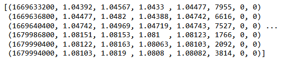
#check
print(eurusd_rates)
#create dataframe
df = pd.DataFrame(eurusd_rates)
データフレームの開始と終了を表示します。
#show dataframe head
df.head()

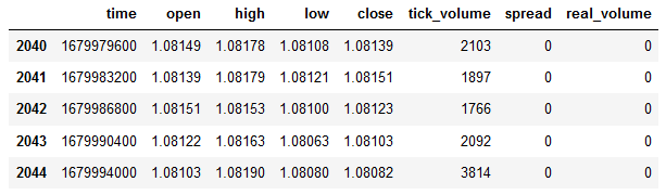
#show dataframe tail
df.tail()
#show dataframe shape (the number of rows and columns in the data set)
df.shape
(2045, 8)
終値のみを選択します。
#prepare close prices only
data = df.filter(['close']).values
データを出力します。
#show close prices
plt.figure(figsize = (18,10))
plt.plot(data,'b',label = 'Original')
plt.xlabel("Hours")
plt.ylabel("Price")
plt.title("EURUSD_H1")
plt.legend()

MinMaxScalerを使用してソース価格データを[0,1]の範囲にスケーリングします。
#scale data using MinMaxScaler
from sklearn.preprocessing import MinMaxScaler
scaler=MinMaxScaler(feature_range=(0,1))
scaled_data = scaler.fit_transform(data)
データの最初の80%が訓練に使用されます。
#training size is 80% of the data
training_size = int(len(scaled_data)*0.80)
print("training size:",training_size)
訓練サイズ:1636
#create train data and check size
train_data_initial = scaled_data[0:training_size,:]
print(len(train_data_initial))
1636
#create test data and check size
test_data_initial= scaled_data[training_size:,:1]
print(len(test_data_initial))
409
次の関数は訓練シーケンスを作成します。
#split a univariate sequence into samples
def split_sequence(sequence, n_steps):
    X, y = list(), list()
    for i in range(len(sequence)):
       #find the end of this pattern
       end_ix = i + n_steps
       #check if we are beyond the sequence
       if end_ix > len(sequence)-1:
          break
       #gather input and output parts of the pattern
       seq_x, seq_y = sequence[i:end_ix], sequence[end_ix]
       X.append(seq_x)
       y.append(seq_y)
    return np.array(X), np.array(y)
セットを構築します。
#split into samples
time_step = 120
x_train, y_train = split_sequence(train_data_initial, time_step)
x_test, y_test = split_sequence(test_data_initial, time_step)
#reshape input to be [samples, time steps, features] which is required for LSTM
x_train =x_train.reshape(x_train.shape[0],x_train.shape[1],1)
x_test = x_test.reshape(x_test.shape[0],x_test.shape[1],1)
訓練とテスト用のテンソル形状:
#show shape of train data
x_train.shape
(1516, 120, 1)
#show shape of test data
x_test.shape
(289, 120, 1)
#import keras libraries for the model
import math
from keras.models import Sequential
from keras.layers import Dense,Activation,Conv1D,MaxPooling1D,Dropout
from keras.layers import LSTM
from keras.utils.vis_utils import plot_model
from keras.metrics import RootMeanSquaredError as rmse
from keras import optimizers
モデルを設定します。
#define the model
model = Sequential()
model.add(Conv1D(filters=256, kernel_size=2,activation='relu',padding = 'same',input_shape=(120,1)))
model.add(MaxPooling1D(pool_size=2))
model.add(LSTM(100, return_sequences = True))
model.add(Dropout(0.3))
model.add(LSTM(100, return_sequences = False))
model.add(Dropout(0.3))
model.add(Dense(units=1, activation = 'sigmoid'))
model.compile(optimizer='adam', loss= 'mse' , metrics = [rmse()])
モデルプロパティを表示します。
#show model
model.summary()

モデル訓練:
#measure time
import time
time_calc_start = time.time()

#fit model with 300 epochs
history=model.fit(x_train,y_train,epochs=300,validation_data=(x_test,y_test),batch_size=32,verbose=1)

#calculate time
fit_time_seconds = time.time() - time_calc_start
print("fit time =",fit_time_seconds," seconds.")
Epoch 1/300
48/48 [==============================] - 8s 49ms/step - loss:0.0129 - root_mean_squared_error:0.1136 - val_loss:0.0065-val_root_mean_squared_error:0.0804
...
Epoch 299/300
48/48 [==============================] - 2s 35ms/step - loss:4.5197e-04-root_mean_squared_error:0.0213 - val_loss:4.2535e-04-val_root_mean_squared_error:0.0206
Epoch 300/300
48/48 [==============================] - 2s 32ms/step - loss:4.2967e-04-root_mean_squared_error:0.0207 - val_loss:4.4040e-04-val_root_mean_squared_error:0.0210
fit time = 467.4918096065521 seconds.
訓練にかかった時間は約8分です。
#show training history keys
history.history.keys()
訓練およびテストデータセットにおける最適化ダイナミクス:
#show iteration-loss graph for training and validation
plt.figure(figsize = (18,10))
plt.plot(history.history['loss'],label='Training Loss',color='b')
plt.plot(history.history['val_loss'],label='Validation-loss',color='g')
plt.xlabel("Iteration")
plt.ylabel("Loss")
plt.title("LOSS")
plt.legend()

#show iteration-rmse graph for training and validation
plt.figure(figsize = (18,10))
plt.plot(history.history['root_mean_squared_error'],label='Training RMSE',color='b')
plt.plot(history.history['val_root_mean_squared_error'],label='Validation-RMSE',color='g')
plt.xlabel("Iteration")
plt.ylabel("RMSE")
plt.title("RMSE")
plt.legend()

#evaluate training data
model.evaluate(x_train,y_train, batch_size = 32)
[0.00029911252204328775,0.01729486882686615]
#evaluate testing data
model.evaluate(x_test,y_test, batch_size = 32)
10/10 [==============================] - 0s 31ms/step - loss:4.4040e-04-root_mean_squared_error:0.0210
[0.00044039846397936344,0.020985672250390053]
訓練データセットに対する予測の形成:
#prediction using training data
train_predict = model.predict(x_train)
plot_y_train = y_train.reshape(-1,1)
訓練間隔の実際のグラフと予測されたグラフを出力します。
#show actual vs predicted (training) graph
plt.figure(figsize=(18,10))
plt.plot(scaler.inverse_transform(plot_y_train),color = 'b', label = 'Original')
plt.plot(scaler.inverse_transform(train_predict),color='red', label = 'Predicted')
plt.title("Prediction Graph Using Training Data")
plt.xlabel("Hours")
plt.ylabel("Price")
plt.legend()
plt.show()

テストデータセットでの予測の形成:
#prediction using testing data
test_predict = model.predict(x_test)
plot_y_test = y_test.reshape(-1,1)
11/11 [==============================] - 0s 11ms/step
メトリックを計算するには、間隔[0,1]からデータを変換する必要があります。繰り返しますが、MinMaxScalerを使用します。
#calculate metrics
from sklearn import metrics
from sklearn.metrics import r2_score
#transform data to real values
value1=scaler.inverse_transform(plot_y_test)
value2=scaler.inverse_transform(test_predict)
#calc score
score = np.sqrt(metrics.mean_squared_error(value1,value2))
print("RMSE         : {}".format(score))
print("MSE          :", metrics.mean_squared_error(value1,value2))
print("R2 score     :",metrics.r2_score(value1,value2))
RMSE:0.0015151631684117558
MSE:2.295719426911551e-06
R2スコア:0.9683533377809039
#show actual vs predicted (testing) graph
plt.figure(figsize=(18,10))
plt.plot(scaler.inverse_transform(plot_y_test),color = 'b',  label = 'Original')
plt.plot(scaler.inverse_transform(test_predict),color='g', label = 'Predicted')
plt.title("Prediction Graph Using Testing Data")
plt.xlabel("Hours")
plt.ylabel("Price")
plt.legend()
plt.show()

モデルをonnxファイルにエクスポートします。
# save model to ONNX
output_path = data_path+"model.eurusd.H1.120.onnx"
onnx_model = tf2onnx.convert.from_keras(model, output_path=output_path)
print(f"model saved to {output_path}")

output_path = file_path+"model.eurusd.H1.120.onnx"
onnx_model = tf2onnx.convert.from_keras(model, output_path=output_path)
print(f"saved model to {output_path}")

# finish
mt5.shutdown()
Pythonスクリプトの完全なコードは、Jupyter Notebookの記事に添付されています。
「A CNN-LSTM-Based Model to Forecast Stock Prices」稿では、CNN-LSTMを使用したモデルで最良の結果R^2=0.9646が得られました。この例では、CNN-LSTMネットワークがR^2=0.9684という最良の結果を生成しました。結果によると、このタイプのモデルは予測問題を効率的に解決できます。
金融務時系列を予測するためにCNN-LSTMモデルを構築および訓練するPythonスクリプトの例を検討しました。
2.MetaTrader 5でモデルを使用する
2.1.始める前に知っておくとよいこと
モデルを作成するには、次の2つの方法があります。OnnxCreateを使用してonnxファイルからモデルを作成するか、OnnxCreateFromBufferを使用してデータ配列からモデルを作成することができます。
ONNXモデルがEAのリソースとして使用されている場合、モデルを変更するたびにEAを再コンパイルする必要があります。
すべてのモデルに完全に定義されたサイズの入力および/または出力テンソルがあるわけではありません。これは通常、パッケージサイズを決定する最初の次元です。モデルを実行する前に、OnnxSetInputShapeおよびOnnxSetOutputShape関数を使用してサイズを明示的に指定する必要があります。モデルの入力データは、モデルの訓練時に行ったのと同じ方法で準備する必要があります。
入力データと出力データについては、モデルで使用されているのと同じ型の配列、行列、および/またはベクトルを使用することをお勧めします。この場合、モデルの実行時にデータを変換する必要はありません。データが必要な型で表現できない場合、データは自動的に変換されます。
OnnxRunを使用して、モデルを推論(実行)します。モデルは複数回実行できます。モデルを使用した後、OnnxRelease関数を使用してモデルを解放します。
2.2.onnxファイルを読み取り、入力と出力に関する情報を取得する
モデルを使用するには、モデルの場所、入力データ型と形状、出力データ型と形状を知る必要があります。以前に作成したスクリプトによると、model.eurusd.H1.120.onnxは、onnxファイルを生成したPythonスクリプトと同じフォルダにあります。入力はfloat32、120の正規化された終値(バッチサイズが1の場合)です。出力はfloat32で、これはモデルによって予測された1つの正規化された価格です。
また、MQL5スクリプトを使用してモデルの入力データと出力データを取得するために、MQL5\Filesフォルダにonnxファイルを作成しました。
//+------------------------------------------------------------------+
//|                                                OnnxModelInfo.mq5 |
//|                                  Copyright 2023, MetaQuotes Ltd. |
//|                                             https://www.mql5.com |
//+------------------------------------------------------------------+
#property copyright "Copyright 2023, MetaQuotes Ltd."
#property link      "https://www.mql5.com"
#property version   "1.00"

#define UNDEFINED_REPLACE 1

//+------------------------------------------------------------------+
//| Script program start function                                    |
//+------------------------------------------------------------------+
void OnStart()
  {
   string file_names[];
   if(FileSelectDialog("Open ONNX model",NULL,"ONNX files (*.onnx)|*.onnx|All files (*.*)|*.*",FSD_FILE_MUST_EXIST,file_names,NULL)<1)
      return;

   PrintFormat("Create model from %s with debug logs",file_names[0]);

   long session_handle=OnnxCreate(file_names[0],ONNX_DEBUG_LOGS);
   if(session_handle==INVALID_HANDLE)
     {
      Print("OnnxCreate error ",GetLastError());
      return;
     }

   OnnxTypeInfo type_info;

   long input_count=OnnxGetInputCount(session_handle);
   Print("model has ",input_count," input(s)");
   for(long i=0; i<input_count; i++)
     {
      string input_name=OnnxGetInputName(session_handle,i);
      Print(i," input name is ",input_name);
      if(OnnxGetInputTypeInfo(session_handle,i,type_info))
         PrintTypeInfo(i,"input",type_info);
     }

   long output_count=OnnxGetOutputCount(session_handle);
   Print("model has ",output_count," output(s)");
   for(long i=0; i<output_count; i++)
     {
      string output_name=OnnxGetOutputName(session_handle,i);
      Print(i," output name is ",output_name);
      if(OnnxGetOutputTypeInfo(session_handle,i,type_info))
         PrintTypeInfo(i,"output",type_info);
     }

   OnnxRelease(session_handle);
  }
//+------------------------------------------------------------------+
//| PrintTypeInfo                                                    |
//+------------------------------------------------------------------+
void PrintTypeInfo(const long num,const string layer,const OnnxTypeInfo& type_info)
  {
   Print("   type ",EnumToString(type_info.type));
   Print("   data type ",EnumToString(type_info.element_type));

   if(type_info.dimensions.Size()>0)
     {
      bool   dim_defined=(type_info.dimensions[0]>0);
      string dimensions=IntegerToString(type_info.dimensions[0]);
      for(long n=1; n<type_info.dimensions.Size(); n++)
        {
         if(type_info.dimensions[n]<=0)
            dim_defined=false;
         dimensions+=", ";
         dimensions+=IntegerToString(type_info.dimensions[n]);
        }
      Print("   shape [",dimensions,"]");
      //--- not all dimensions defined
      if(!dim_defined)
         PrintFormat("   %I64d %s shape must be defined explicitly before model inference",num,layer);
      //--- reduce shape
      uint reduced=0;
      long dims[];
      for(long n=0; n<type_info.dimensions.Size(); n++)
        {
         long dimension=type_info.dimensions[n];
         //--- replace undefined dimension
         if(dimension<=0)
            dimension=UNDEFINED_REPLACE;
         //--- 1 can be reduced
         if(dimension>1)
           {
            ArrayResize(dims,reduced+1);
            dims[reduced++]=dimension;
           }
        }
      //--- all dimensions assumed 1
      if(reduced==0)
        {
         ArrayResize(dims,1);
         dims[reduced++]=1;
        }
      //--- shape was reduced
      if(reduced<type_info.dimensions.Size())
        {
         dimensions=IntegerToString(dims[0]);
         for(long n=1; n<dims.Size(); n++)
           {
            dimensions+=", ";
            dimensions+=IntegerToString(dims[n]);
           }
         string sentence="";
         if(!dim_defined)
            sentence=" if undefined dimension set to "+(string)UNDEFINED_REPLACE;
         PrintFormat("   shape of %s data can be reduced to [%s]%s",layer,dimensions,sentence);
        }
     }
   else
      PrintFormat("no dimensions defined for %I64d %s",num,layer);
  }
//+------------------------------------------------------------------+
ファイル選択ウィンドウで、MQL5\Filesに保存されているonnxファイルを選択し、OnnxCreateを使用してファイルからモデルを作成し、次の情報を取得しました。
Create model from model.eurusd.H1.120.onnx with debug logs
ONNX: Creating and using per session threadpools since use_per_session_threads_ is true
ONNX: Dynamic block base set to 0
ONNX: Initializing session.
ONNX: Adding default CPU execution provider.
ONNX: Total shared scalar initializer count: 0
ONNX: Total fused reshape node count: 0
ONNX: Removing NodeArg 'Gather_out0'. It is no longer used by any node.
ONNX: Removing NodeArg 'Gather_token_1_out0'. It is no longer used by any node.
ONNX: Total shared scalar initializer count: 0
ONNX: Total fused reshape node count: 0
ONNX: Removing initializer 'sequential/conv1d/Conv1D/ExpandDims_1:0'. It is no longer used by any node.
ONNX: Use DeviceBasedPartition as default
ONNX: Saving initialized tensors.
ONNX: Done saving initialized tensors
ONNX: Session successfully initialized.
model has 1 input(s)
0 input name is conv1d_input
   type ONNX_TYPE_TENSOR
   data type ONNX_DATA_TYPE_FLOAT
   shape [-1, 120, 1]
   0 input shape must be defined explicitly before model inference
   shape of input data can be reduced to [120] if undefined dimension set to 1
model has 1 output(s)
0 output name is dense
   type ONNX_TYPE_TENSOR
   data type ONNX_DATA_TYPE_FLOAT
   shape [-1, 1]
   0 output shape must be defined explicitly before model inference
   shape of output data can be reduced to [1] if undefined dimension set to 1
デバッグモードが有効になっているので
long session_handle=OnnxCreate(file_names[0],ONNX_DEBUG_LOGS);
ONNXプレフィックスを持つログがあります。
モデルには実際には1つの入力と1つの出力があることがわかります。ここで、入力テンソルの最初の次元と出力テンソルの最初の次元は定義されていません。これらのディメンションがバッチサイズの原因であると想定されます。したがって、モデルを推論する前に、使用するサイズ(OnnxSetInputShapeおよびOnnxSetOutputShape)を明示的に指定する必要があります。通常、モデルに入力されるデータセットは1つだけです。詳細な例は、次の段落「取引EAでのONNXモデルの使用例」に記載されています。
データを準備するとき、次元が[1,120,1]の配列を使用する必要はありません。1次元配列または120要素のベクトルを入力できます。
2.3.取引EAでのONNXモデルの使用例
宣言と定義
#include <Trade\Trade.mqh>

input double InpLots = 1.0;    // Lots amount to open position

#resource "Python/model.120.H1.onnx" as uchar ExtModel[]

#define SAMPLE_SIZE 120

long     ExtHandle=INVALID_HANDLE;
int      ExtPredictedClass=-1;
datetime ExtNextBar=0;
datetime ExtNextDay=0;
float    ExtMin=0.0;
float    ExtMax=0.0;
CTrade   ExtTrade;

//--- price movement prediction
#define PRICE_UP   0
#define PRICE_SAME 1
#define PRICE_DOWN 2
OnInit関数
//+------------------------------------------------------------------+
//| Expert initialization function                                   |
//+------------------------------------------------------------------+
int OnInit()
  {
   if(_Symbol!="EURUSD" || _Period!=PERIOD_H1)
     {
      Print("model must work with EURUSD,H1");
      return(INIT_FAILED);
     }

//--- create a model from static buffer
   ExtHandle=OnnxCreateFromBuffer(ExtModel,ONNX_DEFAULT);
   if(ExtHandle==INVALID_HANDLE)
     {
      Print("OnnxCreateFromBuffer error ",GetLastError());
      return(INIT_FAILED);
     }

//--- since not all sizes defined in the input tensor we must set them explicitly
//--- first index - batch size, second index - series size, third index - number of series (only Close)
   const long input_shape[] = {1,SAMPLE_SIZE,1};
   if(!OnnxSetInputShape(ExtHandle,ONNX_DEFAULT,input_shape))
     {
      Print("OnnxSetInputShape error ",GetLastError());
      return(INIT_FAILED);
     }

//--- since not all sizes defined in the output tensor we must set them explicitly
//--- first index - batch size, must match the batch size of the input tensor
//--- second index - number of predicted prices (we only predict Close)
   const long output_shape[] = {1,1};
   if(!OnnxSetOutputShape(ExtHandle,0,output_shape))
     {
      Print("OnnxSetOutputShape error ",GetLastError());
      return(INIT_FAILED);
     }
//---
   return(INIT_SUCCEEDED);
  }
現在の銘柄/期間データを使用するため、EURUSD、H1のみを使用します。
私たちのモデルはリソースとしてEAに含まれています。EAは完全に自己完結型であり、外部のonnxファイルを読み取る必要はありません。リソース配列からモデルが作成されます。
入力および出力のデータ形状は、明示的に定義する必要があります。
OnTick関数:
//+------------------------------------------------------------------+
//| Expert tick function                                             |
//+------------------------------------------------------------------+
void OnTick()
  {
//--- check new day
   if(TimeCurrent()>=ExtNextDay)
     {
      GetMinMax();
      //--- set next day time
      ExtNextDay=TimeCurrent();
      ExtNextDay-=ExtNextDay%PeriodSeconds(PERIOD_D1);
      ExtNextDay+=PeriodSeconds(PERIOD_D1);
     }

//--- check new bar
   if(TimeCurrent()<ExtNextBar)
      return;
//--- set next bar time
   ExtNextBar=TimeCurrent();
   ExtNextBar-=ExtNextBar%PeriodSeconds();
   ExtNextBar+=PeriodSeconds();
//--- check min and max
   double close=iClose(_Symbol,_Period,0);
   if(ExtMin>close)
      ExtMin=close;
   if(ExtMax<close)
      ExtMax=close;

//--- predict next price
   PredictPrice();
//--- check trading according to prediction
   if(ExtPredictedClass>=0)
      if(PositionSelect(_Symbol))
         CheckForClose();
      else
         CheckForOpen();
  }
新しい1日の始まりを定義します。1日の始まりは、120時間系列の価格を正規化するために、120日系列の安値と高値を更新するために使用されます。モデルは、入力データを準備するときに従わなければならないこれらの条件下で訓練されました。
//+------------------------------------------------------------------+
//| Get minimal and maximal Close for last 120 days                  |
//+------------------------------------------------------------------+
void GetMinMax(void)
  {
   vectorf close;
   close.CopyRates(_Symbol,PERIOD_D1,COPY_RATES_CLOSE,0,SAMPLE_SIZE);
   ExtMin=close.Min();
   ExtMax=close.Max();
  }
必要に応じて、1日を通してLowとHighを変更できます。
次は予測関数です。
//+------------------------------------------------------------------+
//| Predict next price                                               |
//+------------------------------------------------------------------+
void PredictPrice(void)
  {
   static vectorf output_data(1);            // vector to get result
   static vectorf x_norm(SAMPLE_SIZE);       // vector for prices normalize

//--- check for normalization possibility
   if(ExtMin>=ExtMax)
     {
      ExtPredictedClass=-1;
      return;
     }
//--- request last bars
   if(!x_norm.CopyRates(_Symbol,_Period,COPY_RATES_CLOSE,1,SAMPLE_SIZE))
     {
      ExtPredictedClass=-1;
      return;
     }
   float last_close=x_norm[SAMPLE_SIZE-1];
//--- normalize prices
   x_norm-=ExtMin;
   x_norm/=(ExtMax-ExtMin);
//--- run the inference
   if(!OnnxRun(ExtHandle,ONNX_NO_CONVERSION,x_norm,output_data))
     {
      ExtPredictedClass=-1;
      return;
     }
//--- denormalize the price from the output value
   float predicted=output_data[0]*(ExtMax-ExtMin)+ExtMin;
//--- classify predicted price movement
   float delta=last_close-predicted;
   if(fabs(delta)<=0.00001)
      ExtPredictedClass=PRICE_SAME;
   else
     {
      if(delta<0)
         ExtPredictedClass=PRICE_UP;
      else
         ExtPredictedClass=PRICE_DOWN;
     }
  }
まず、正規化できるかどうかを確認します。正規化は、MinMaxScalerPython関数のように実装されます。
#scale data
from sklearn.preprocessing import MinMaxScaler
scaler=MinMaxScaler(feature_range=(0,1))
scaled_data = scaler.fit_transform(data)
したがって、正規化コードは非常に単純で簡単です。
入力データと結果を受け取るためのベクトルは、静的として編成されます。これにより、プログラムの存続期間全体にわたって存在する再配置不可能なバッファが保証されます。したがって、ONNXモデルの入力テンソルと出力テンソルは、モデルを実行するたびに再作成されるわけではありません。
主要関数はOnnxRunです。ONNX_NO_CONVERSIONフラグは、MQL5float型がONNX_DATA_TYPE_FLOATに正確に対応するため、入力および出力データを変換してはならないことを示します。ONNX_DEBUGフラグが設定されていません。
その後、取得したデータを予測価格に非正規化し、価格が上がるか下がるか、変わらないかのクラスを決定します。
取引戦略は簡単です。各時間の開始時に、その時間の終わりの価格予測を確認します。予想価格が上がれば、買います。モデルが下向きの動きを予測する場合、売ります。
//+------------------------------------------------------------------+
//| Check for open position conditions                               |
//+------------------------------------------------------------------+
void CheckForOpen(void)
  {
   ENUM_ORDER_TYPE signal=WRONG_VALUE;
//--- check signals
   if(ExtPredictedClass==PRICE_DOWN)
      signal=ORDER_TYPE_SELL;    // sell condition
   else
     {
      if(ExtPredictedClass==PRICE_UP)
         signal=ORDER_TYPE_BUY;  // buy condition
     }

//--- open position if possible according to signal
   if(signal!=WRONG_VALUE && TerminalInfoInteger(TERMINAL_TRADE_ALLOWED))
     {
      double price;
      double bid=SymbolInfoDouble(_Symbol,SYMBOL_BID);
      double ask=SymbolInfoDouble(_Symbol,SYMBOL_ASK);
      if(signal==ORDER_TYPE_SELL)
         price=bid;
      else
         price=ask;
      ExtTrade.PositionOpen(_Symbol,signal,InpLots,price,0.0,0.0);
     }
  }
//+------------------------------------------------------------------+
//| Check for close position conditions                              |
//+------------------------------------------------------------------+
void CheckForClose(void)
  {
   bool bsignal=false;
//--- position already selected before
   long type=PositionGetInteger(POSITION_TYPE);
//--- check signals
   if(type==POSITION_TYPE_BUY && ExtPredictedClass==PRICE_DOWN)
      bsignal=true;
   if(type==POSITION_TYPE_SELL && ExtPredictedClass==PRICE_UP)
      bsignal=true;

//--- close position if possible
   if(bsignal && TerminalInfoInteger(TERMINAL_TRADE_ALLOWED))
     {
      ExtTrade.PositionClose(_Symbol,3);
      //--- open opposite
      CheckForOpen();
     }
  }
それでは、ストラテジーテスターでEAのパフォーマンスを確認してみましょう。年初からEAをテストするには、以前のデータを使用してモデルを訓練する必要があります。そのため、未使用の部分を削除し、訓練の終了日をテスト期間と重ならないように変更するなど、Pythonスクリプトをわずかに変更しました。
ONNX.eurusd.H1.120.Training.pyスクリプトはPythonサブフォルダにあり、MetaEditorで直接実行されます。結果のONNXモデルは同じPythonサブフォルダに保存され、EAのコンパイル中にリソースとして使用されます。
# Copyright 2023, MetaQuotes Ltd.
# https://www.mql5.com

# python libraries
import MetaTrader5 as mt5
import tensorflow as tf
import numpy as np
import pandas as pd
import tf2onnx

# input parameters
inp_model_name = "model.eurusd.H1.120.onnx"
inp_history_size = 120

if not mt5.initialize():
    print("initialize() failed, error code =",mt5.last_error())
    quit()

# we will save generated onnx-file near our script to use as resource
from sys import argv
data_path=argv[0]
last_index=data_path.rfind("\\")+1
data_path=data_path[0:last_index]
print("data path to save onnx model",data_path)

# set start and end dates for history data
from datetime import timedelta, datetime
#end_date = datetime.now()
end_date = datetime(2023, 1, 1, 0)
start_date = end_date - timedelta(days=inp_history_size)

# print start and end dates
print("data start date =",start_date)
print("data end date =",end_date)

# get rates
eurusd_rates = mt5.copy_rates_range("EURUSD", mt5.TIMEFRAME_H1, start_date, end_date)

# create dataframe
df = pd.DataFrame(eurusd_rates)

# get close prices only
data = df.filter(['close']).values

# scale data
from sklearn.preprocessing import MinMaxScaler
scaler=MinMaxScaler(feature_range=(0,1))
scaled_data = scaler.fit_transform(data)

# training size is 80% of the data
training_size = int(len(scaled_data)*0.80)
print("Training_size:",training_size)
train_data_initial = scaled_data[0:training_size,:]
test_data_initial = scaled_data[training_size:,:1]

# split a univariate sequence into samples
def split_sequence(sequence, n_steps):
    X, y = list(), list()
    for i in range(len(sequence)):
       # find the end of this pattern
       end_ix = i + n_steps
       # check if we are beyond the sequence
       if end_ix > len(sequence)-1:
          break
       # gather input and output parts of the pattern
       seq_x, seq_y = sequence[i:end_ix], sequence[end_ix]
       X.append(seq_x)
       y.append(seq_y)
    return np.array(X), np.array(y)

# split into samples
time_step = inp_history_size
x_train, y_train = split_sequence(train_data_initial, time_step)
x_test, y_test = split_sequence(test_data_initial, time_step)

# reshape input to be [samples, time steps, features] which is required for LSTM
x_train =x_train.reshape(x_train.shape[0],x_train.shape[1],1)
x_test = x_test.reshape(x_test.shape[0],x_test.shape[1],1)

# define model
from keras.models import Sequential
from keras.layers import Dense, Activation, Conv1D, MaxPooling1D, Dropout, Flatten, LSTM
from keras.metrics import RootMeanSquaredError as rmse
model = Sequential()
model.add(Conv1D(filters=256, kernel_size=2, activation='relu',padding = 'same',input_shape=(inp_history_size,1)))
model.add(MaxPooling1D(pool_size=2))
model.add(LSTM(100, return_sequences = True))
model.add(Dropout(0.3))
model.add(LSTM(100, return_sequences = False))
model.add(Dropout(0.3))
model.add(Dense(units=1, activation = 'sigmoid'))
model.compile(optimizer='adam', loss= 'mse' , metrics = [rmse()])

# model training for 300 epochs
history = model.fit(x_train, y_train, epochs = 300 , validation_data = (x_test,y_test), batch_size=32, verbose=2)

# evaluate training data
train_loss, train_rmse = model.evaluate(x_train,y_train, batch_size = 32)
print(f"train_loss={train_loss:.3f}")
print(f"train_rmse={train_rmse:.3f}")

# evaluate testing data
test_loss, test_rmse = model.evaluate(x_test,y_test, batch_size = 32)
print(f"test_loss={test_loss:.3f}")
print(f"test_rmse={test_rmse:.3f}")

# save model to ONNX
output_path = data_path+inp_model_name
onnx_model = tf2onnx.convert.from_keras(model, output_path=output_path)
print(f"saved model to {output_path}")

# finish
mt5.shutdown()
ONNXモデルベースのEAのテスト
ここで、ストラテジーテスターの履歴データでEAをテストしてみましょう。モデルの訓練に使用したのと同じパラメータを指定します(:EURUSD銘柄とH1時間枠)。
テスト間隔には訓練期間は含まれません。年初(2023年1月1日)から開始されます。

ストラテジーによれば、シグナルは各時間の開始時に1回チェックされます(EAは新しいバーの出現を監視します)。したがって、ティックモデリングモードは重要ではありません。OnTickはテスターでバーごとに1回処理されます。
//+------------------------------------------------------------------+
//| Expert tick function                                             |
//+------------------------------------------------------------------+
void OnTick()
  {
//--- check new day
   if(TimeCurrent()>=ExtNextDay)
     {
      GetMinMax();
      //--- set next day time
      ExtNextDay=TimeCurrent();
      ExtNextDay-=ExtNextDay%PeriodSeconds(PERIOD_D1);
      ExtNextDay+=PeriodSeconds(PERIOD_D1);
     }

//--- check new bar
   if(TimeCurrent()<ExtNextBar)
      return;
//--- set next bar time
   ExtNextBar=TimeCurrent();
   ExtNextBar-=ExtNextBar%PeriodSeconds();
   ExtNextBar+=PeriodSeconds();
//--- check min and max
   float close=(float)iClose(_Symbol,_Period,0);
   if(ExtMin>close)
      ExtMin=close;
   if(ExtMax<close)
      ExtMax=close;

//--- predict next price
   PredictPrice();
//--- check trading according to prediction
   if(ExtPredictedClass>=0)
      if(PositionSelect(_Symbol))
         CheckForClose();
      else
         CheckForOpen();
  }
この処理により、3か月の期間テストはわずか数秒で完了します。結果は以下のとおりです。

ここで、シグナルによるポジションオープンとストップロス(SL)またはテイクプロフィット(TP)による決済を可能にするように取引戦略を変更しましょう。
input double InpLots       = 1.0;    // Lots amount to open position
input bool   InpUseStops   = true;   // Use stops in trading
input int    InpTakeProfit = 500;    // TakeProfit level
input int    InpStopLoss   = 500;    // StopLoss level

//+------------------------------------------------------------------+
//| Check for open position conditions                               |
//+------------------------------------------------------------------+
void CheckForOpen(void)
  {
   ENUM_ORDER_TYPE signal=WRONG_VALUE;
//--- check signals
   if(ExtPredictedClass==PRICE_DOWN)
      signal=ORDER_TYPE_SELL;    // sell condition
   else
     {
      if(ExtPredictedClass==PRICE_UP)
         signal=ORDER_TYPE_BUY;  // buy condition
     }

//--- open position if possible according to signal
   if(signal!=WRONG_VALUE && TerminalInfoInteger(TERMINAL_TRADE_ALLOWED))
     {
      double price,sl=0,tp=0;
      double bid=SymbolInfoDouble(_Symbol,SYMBOL_BID);
      double ask=SymbolInfoDouble(_Symbol,SYMBOL_ASK);
      if(signal==ORDER_TYPE_SELL)
        {
         price=bid;
         if(InpUseStops)
           {
            sl=NormalizeDouble(bid+InpStopLoss*_Point,_Digits);
            tp=NormalizeDouble(ask-InpTakeProfit*_Point,_Digits);
           }
        }
      else
        {
         price=ask;
         if(InpUseStops)
           {
            sl=NormalizeDouble(ask-InpStopLoss*_Point,_Digits);
            tp=NormalizeDouble(bid+InpTakeProfit*_Point,_Digits);
           }
        }
      ExtTrade.PositionOpen(_Symbol,signal,InpLots,price,sl,tp);
     }
  }
//+------------------------------------------------------------------+
//| Check for close position conditions                              |
//+------------------------------------------------------------------+
void CheckForClose(void)
  {
//--- position should be closed by stops
   if(InpUseStops)
      return;

   bool bsignal=false;
//--- position already selected before
   long type=PositionGetInteger(POSITION_TYPE);
//--- check signals
   if(type==POSITION_TYPE_BUY && ExtPredictedClass==PRICE_DOWN)
      bsignal=true;
   if(type==POSITION_TYPE_SELL && ExtPredictedClass==PRICE_UP)
      bsignal=true;

//--- close position if possible
   if(bsignal && TerminalInfoInteger(TERMINAL_TRADE_ALLOWED))
     {
      ExtTrade.PositionClose(_Symbol,3);
      //--- open opposite
      CheckForOpen();
     }
  }
InpUseStops=trueは、SLとTPレベルがポジションを開くときに設定されることを意味します。

同じ期間のSL/TPレベルでのテスト結果:

EAの完全なソースコードと訓練済みモデル(2023年の初めまで)は、添付ファイルにあります。
結論
この記事では、MQL5プログラムでONNXモデルを使用するのに難しいことは何もないことが分かります。実際、モデルの適用は最も簡単な部分ですが、適切なONNXモデルを取得するのははるかに困難です。
この記事で使用されているモデルは、MQL5言語を使用してONNXモデルを操作する方法を示すために、デモンストレーションのみを目的として提供されているので、ご注意ください。この記事で紹介するEAは、実際の取引を目的としたものではありません。
MetaQuotes Ltdによってロシア語から翻訳されました。
元の記事: https://www.mql5.com/ru/articles/12373
警告: これらの資料についてのすべての権利はMetaQuotes Ltd.が保有しています。これらの資料の全部または一部の複製や再プリントは禁じられています。

- 無料取引アプリ
- 8千を超えるシグナルをコピー
- 金融ニュースで金融マーケットを探索
ラベルはクラス値を含み、テンソルは確率を含む。したがって、出力次元は本来2,2ですが、構造体が返されるので、1を置くべきです。
ありがとうございました。
ありがとう
それは、あなたが尊重しない前処理は、そのためにあるのです :) 籾殻から穀粒を最初に分離し、分離された穀粒を予測するためにそれを訓練する。
前処理がうまくいけば、出力もゴミのようなものにはならない。
このスクリプトを新しいバージョンのpython(3.10-3.12)で実行できるように修正できる可能性はありますか?
3.9で実行させようとすると問題が山積みです。
tx