
Overcoming ONNX Integration Challenges

Introduction
ONNX (Open Neural Network Exchange) revolutionizes the way we make sophisticated AI-based mql5 programs. This new technology to MetaTrader 5 is the way forward to machine learning as it shows a lot of promise like no other for its purpose however, ONNX comes with a couple of challenges that can give you headaches if you have no clue how to solve them whatsoever.
If you deploy a simple AI technique like a feedforward neural network you might not be able to find the deployment process that problematic but since most real-life projects are much more complex you might be required to do a lot of things such as extracting time-series data, preprocess and transform the big data to reduce its dimensions not to mention when you have to use several models in one big project deploying ONNX models, in situations like this deploying ONNX can become complicated.
ONNX is a self-sufficient tool that comes with the ability to store an AI model only. It doesn't come with everything in the box necessary to run the trained models on the other end, it is up to you to figure out how are you going to deploy your final ONNX models. In this article, we will discuss the three challenges which are scaling & normalizing the data, introducing dimension reduction to the model and, overcoming the challenge of deploying ONNX models for time-series predictions.

This article assumes you have a basic understanding of machine learning and AI theory, and that you have at least tried to use ONNX models in mql5 once or twice.
Overcoming the Data Pre-processing Challenges
In the context of machine-learning, Data-processing refers to the process of transforming the values of features in your dataset to a specific range. This transformation aims to achieve a more consistent representation of the data for your machine learning model. The scaling process is very crucial for several reasons;
It Improves Machine Learning Model(s) Performance: Many machine learning algorithms, especially distance-based ones like K-Nearest Neighbors (KNN) and Support Vector Machines (SVMs), rely on calculating distances between data points. If features have vastly different scales (e.g., one feature in thousands, another in tenths), the features with larger scales will dominate the distance calculations, leading to suboptimal performance. Scaling puts all features in a similar range, allowing the model to focus on the actual relationships between the data points.
Faster Training Convergence: Gradient descent-based optimization algorithms, commonly used in neural networks and other models, take steps toward the optimal solution based on the gradients of the loss function. When features have different scales, the gradients can also have vastly different magnitudes, making it harder for the optimizer to find the minimum efficiently. Scaling helps gradients have a more consistent range, leading to faster convergence.
It Ensures Stability of Numerical Operations: Some machine learning algorithms involve calculations that can become unstable with features of significantly different scales. Scaling helps prevent these numerical issues and ensures the model performs calculations accurately.
Common Scaling Techniques:
- Normalization (Min-Max Scaling): This technique scales features to a specific range (often 0 to 1 or -1 to 1).
- Standardization (Z-score normalization): This technique centers the data by subtracting the mean from each feature and then scales it by dividing it by the standard deviation.
As crucial as this normalization process is, not many sources online explain the right way to do it. The same scaling technique and its parameters used for the training data must be applied to the test data and when deploying the model.
Using the same scaler analogy: Imagine you have a feature representing "income" in your training data. The scaler learns the minimum and maximum income values (or mean and standard deviation for standardization) during training. If you use a different scaler on the testing data, it might encounter income values outside the range it saw during training. This can lead to unexpected scaling and introduce inconsistencies between training and testing data.
Using the same parameters for the scaler analogy: Imagine a ruler used to measure height. If you use a different ruler marked with different units (inches vs. centimeters) for training and testing, your measurements wouldn't be comparable. Similarly, using different scalers on training and testing data disrupts the frame of reference the model learned during training.
In essence, using the same scaler ensures the model consistently sees data during both training and testing, leading to more reliable and interpretable results.
from sklearn.preprocessing import MinMaxScaler, StandardScaler
import numpy as np

# Example data
data = np.array([[1000, 2], [500, 1], [2000, 4], [800, 3]])

# Create a MinMaxScaler object
scaler_minmax = MinMaxScaler()

# Fit the scaler on the training data (learn min/max values)
scaler_minmax.fit(data)

# Transform the data using the fitted scaler
data_scaled_minmax = scaler_minmax.transform(data)

print("Original data:\n", data)
print("\nMin Max Scaled data:\n", data_scaled_minmax)
However, things become challenging once you want to use the trained model in the MQL5 language. Despite there being various ways you can save the scaler in Python it will be challenging to extract it in Meta editor since Python has its fancy ways of storing objects and making the process easier than it is in other programming languages. The best thing to do would be to pre-process the data in MQL5, save the scaler, and save the scaled data in a CSV file that we are going to read using Python code.
Below is the roadmap for pre-processing the data:
- Collect the data from the market & Scale it
- Save the scaler
- Save the scaled data to a CSV file
01: Collecting data from the Market & Scaling it
We are going to collect Open, High, Low, and Close rates for 1000 bars from a daily timeframe then we create a pattern recognition problem by assigning the bullish pattern whenever the price closed above where it opened and a bearish signal otherwise. By training the LSTM AI model on this pattern we are trying to get it to understand what contributes to these patterns so that once it is well trained it can be capable of providing us the trading signal.
Inside ONNX collect data script:
We'll start by including the libraries we need:
#include <MALE5\preprocessing.mqh> //This library contains the normalization techniques for machine learning
#include <MALE5\MatrixExtend.mqh>

StandardizationScaler scaler; //We want to use z-normalization/standardization technique for this project
Then we need to collect the price information.
input int data_size = 10000; //number of bars to collect for our dataset

MqlRates rates[];
//+------------------------------------------------------------------+
//| Script program start function                                    |
//+------------------------------------------------------------------+
void OnStart()
  {
//--- vector.CopyRates is lacking we are going to copy rates in normal way

   ArraySetAsSeries(rates, true);
   if (CopyRates(Symbol(), PERIOD_D1, 1, data_size, rates)<-1)
     {
       printf("Failed to collect data Err=%d",GetLastError());
       return;
     }


   matrix OHLC(data_size, 4);
   for (int i=0; i<data_size; i++) //Get OHLC values and save them to a matrix
     {
       OHLC[i][0] = rates[i].open;
       OHLC[i][1] = rates[i].high;
       OHLC[i][2] = rates[i].low;

        if (rates[i].close>rates[i].open)
          OHLC[i][3] = 1; //Buy signal
        else if (rates[i].close<rates[i].open)
          OHLC[i][3] = 0; //sell signal
     }

//---
  }
Remember! Scaling is for the independent variables that is why we split the data matrix into the x and y matrix and vector respectively in order to get the x matrix that we can scale the columns.
   matrix x;
   vector y;
   MatrixExtend::XandYSplitMatrices(OHLC, x, y);  //WE split the data into x and y | The last column in the matrix will be assigned to the y vector

//--- Standardize the data

   x = scaler.fit_transform(x);
02: Saving the Scaler
As said earlier, we need to save the scaler for later use.
   if (!scaler.save(Symbol()+"-SCALER"))
      return;
After this code snippet is run a folder with binary files will be created. These two files contains the parameters for the Standardization scaler we will see later how you can use these parameters to load the saved scaler instance.

03: Saving the scaled data to a CSV file
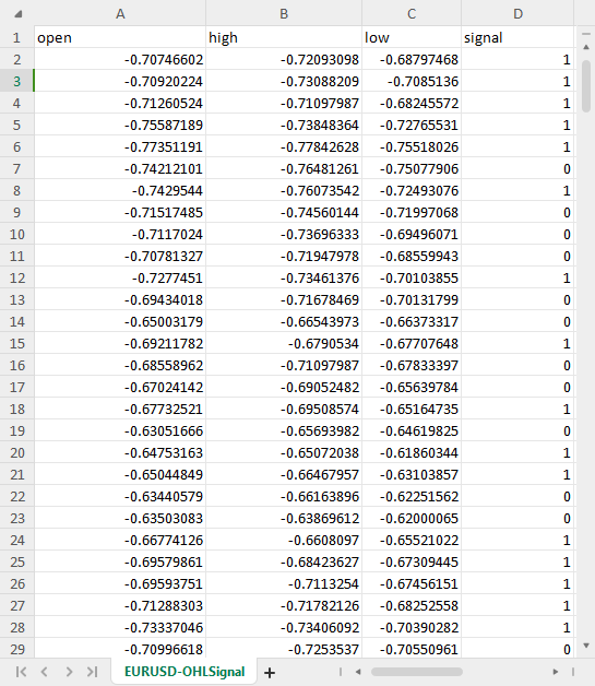
Last but not least, we need to save the scaled data in a CSV file that we can later use in Python code.OHLC = MatrixExtend::concatenate(x, y); //We apped the y column to the scaled x matrix, this is the opposite of XandYsplitMatrices function if (!MatrixExtend::WriteCsv(Symbol()+"-OHLSignal.csv",OHLC,"open,high,low,signal",false,8)) { DebugBreak(); return; }
Outcome:
Overcoming Time Series Data Challenges
There are some studies suggesting time-series deep learning models such as GRU, LSTM, and RNN are better at making predictions in the stock market compared to other models, Due to their ability to understand patterns over a certain period of time, Most algorithmic traders in the data science community are tuned to these particular models including myself.
It turns out that there are some additional lines of code you might be required to write to prepare the data to be suitable for Time series predictions using these models.
If you have worked with Time series models once you probably have seen similar function or code to this:
def get_sequential_data(data, time_step):
    if dataset.empty is True:
      print("Failed to create sequences from an empty dataset")
      return

    Y = data.iloc[:, -1].to_numpy() # get the last column from the dataset and assign it to y numpy 1D array
    X = data.iloc[:, :-1].to_numpy() # Get all the columns from data array except the last column, assign them to x numpy 2D array

    X_reshaped = []
    Y_reshaped = []

    for i in range(len(Y) - time_step + 1):
        X_reshaped.append(X[i:i + time_step])
        Y_reshaped.append(Y[i + time_step - 1])

    return np.array(X_reshaped), np.array(Y_reshaped)
This function is very crucial to Time series models like the LSTM it performs data preparation by:
- Splitting the data into sequences of a fixed size (time_step).
- Separating features (past information) from targets (predicted value).
- Reshaping the data into a format suitable for LSTM models.
This data preparation helps to provide the LSTM model with the most relevant information in a structured way, leading to faster training, better memory management, and potentially improved predictions accuracy.
While LSTMs can handle sequences, real-time data introduces a continuous stream of information. You still need to define a time window of past data for the model to consider when making predictions. This makes this function necessary not only in training and testing but also for real-time predictions. We won't need the y arrays, but we do need to have the code for reshaping the x array. We will be making real-time predictions in MetaTrader 5, right? We need to make a similar function to this in mql5.
Before that let us check the dimensions of x and y Numpy arrays returned by the get_sequential_data function when the time step value was 7.
X_reshaped, Y_reshaped = get_sequential_data(dataset, step_size)

print(f"x_shape{X_reshaped.shape} y_shape{Y_reshaped.shape}")
Outputs:
x_shape(9994, 7, 3) y_shape(9994,)
The returned x array is a 3D array in other words a Tensor while the returned y data is a 1D matrix in other words a vector, We need to consider this while making a similar function in mql5.
Now let us make a simple class with the name CTSDataProcessor:
class CTSDataProcessor
  {
CTensors *tensor_memory[]; //Tensor objects may be hard to track in memory once we return them from a function, this keeps track of them
bool xandysplit;

public:
                     CTSDataProcessor (void);
                    ~CTSDataProcessor (void);

                     CTensors *extract_timeseries_data(const matrix<double> &x, const int time_step); //for real time predictions
                     CTensors *extract_timeseries_data(const matrix<double> &MATRIX, vector &y, const int time_step); //for training and testing purposes
  };
The two functions with similar names extract_timeseries_data do similar work except one does not return the y vector, it will be used for real-time predictions.
CTSDataProcessor ::CTSDataProcessor (void)
 {
   xandysplit = true; //by default obtain the y vector also
 }
//+------------------------------------------------------------------+
//|                                                                  |
//+------------------------------------------------------------------+
CTensors *CTSDataProcessor ::extract_timeseries_data(const matrix<double> &x,const int time_step)
 {
  CTensors *timeseries_tensor;
  timeseries_tensor = new CTensors(0);
  ArrayResize(tensor_memory, 1);
  tensor_memory[0] = timeseries_tensor;

  xandysplit = false; //In this function we do not obtain the y vector

  vector y;
  timeseries_tensor = extract_timeseries_data(x, y, time_step);

  xandysplit = true; //restore the original condition

  return timeseries_tensor;
 }
//+------------------------------------------------------------------+
//|                                                                  |
//+------------------------------------------------------------------+
CTensors *CTSDataProcessor ::extract_timeseries_data(const matrix &MATRIX, vector &y,const int time_step)
 {
  CTensors *timeseries_tensor;
  timeseries_tensor = new CTensors(0);
  ArrayResize(tensor_memory, 1);
  tensor_memory[0] = timeseries_tensor;

  matrix<double> time_series_data = {};
  matrix x = {}; //store the x variables converted to timeseries
  vector y_original = {};
  y.Init(0);

  if (xandysplit) //if we are required to obtain the y vector also split the given matrix into x and y
     if (!MatrixExtend::XandYSplitMatrices(MATRIX, x, y_original))
       {
         printf("%s failed to split the x and y matrices in order to make a tensor",__FUNCTION__);
         return timeseries_tensor;
       }

  x = xandysplit ? x : MATRIX;

  for (ulong sample=0; sample<x.Rows(); sample++) //Go throught all the samples
    {
      matrix<double> time_series_matrix = {};
      vector<double> timeseries_y(1);

      for (ulong time_step_index=0; time_step_index<(ulong)time_step; time_step_index++)
        {
            if (sample + time_step_index >= x.Rows())
                break;

             time_series_matrix = MatrixExtend::concatenate(time_series_matrix, x.Row(sample+time_step_index), 0);

             if (xandysplit)
               timeseries_y[0] = y_original[sample+time_step_index]; //The last value in the column is assumed to be a y value so it gets added to the y vector
        }

      if (time_series_matrix.Rows()<(ulong)time_step)
        continue;

        timeseries_tensor.Append(time_series_matrix);

        if (xandysplit)
         y = MatrixExtend::concatenate(y, timeseries_y);
    }

   return timeseries_tensor;
 }
Now inside an Expert advisor named ONNX challenges EA let's try to use these functions to extract the Time series data:
#include <Timeseries Deep Learning\tsdataprocessor.mqh>

input int time_step_ = 7;
//it is very important the time step value matches the one used during training in  a python script


CTSDataProcessor ts_dataprocessor;
CTensors *ts_data_tensor;
//+------------------------------------------------------------------+
//| Expert initialization function                                   |
//+------------------------------------------------------------------+
int OnInit()
  {
//---

   if (!onnx.Init(lstm_model))
     return INIT_FAILED;

   string headers;
   matrix data = MatrixExtend::ReadCsv("EURUSD-OHLSignal.csv",headers); //let us open the same data so that we don't get confused along the way

   matrix x;
   vector y;

   ts_data_tensor = ts_dataprocessor.extract_timeseries_data(data, y, time_step_);

   printf("x_shape %s y_shape (%d,)",ts_data_tensor.shape(),y.Size());
 }
Outputs:
GD      0       07:21:14.710    ONNX challenges EA (EURUSD,H1)  Warning: CTensors::shape assumes all matrices in the tensor have the same size
IG      0       07:21:14.710    ONNX challenges EA (EURUSD,H1)  x_shape (9994, 7, 3) y_shape (9994,)
Great we got the same dimensions as in the Python code,
The purpose of ONNX is to get a machine learning model built in one language to function well if not the same in the other language, this means if I build a model in Python and run it there the accuracy and precision it provides me there should be nearly the same one that will be provided in another language, in this case, MQL5 language when the same data was used without conversion.
If this is the case, Before you use the ONNX model in MQL5 you need to check if you got everything right by testing the model on the same data on both platforms to see if it provides the same accuracy. Let us test this model.
I made the LSTM model with 10 neurons in the input layer and the single hidden layer in the network, I assigned the Adam optimizer to the learning progress.
from keras.optimizers import Adam
from keras.callbacks import EarlyStopping

learning_rate = 1e-3
patience = 5 #if this number of epochs validation loss is unchanged stop the process


model = Sequential()

model.add(LSTM(units=10, input_shape=(step_size, dataset.shape[1]-1))) #Input layer
model.add(Dense(units=10, activation='relu', kernel_initializer='he_uniform'))
model.add(Dropout(0.3))
model.add(Dense(units=len(classes_in_data), activation = 'softmax')) #last layer outputs = classes in data

model.compile(optimizer=Adam(learning_rate=learning_rate), loss="binary_crossentropy", metrics=['accuracy'])
Outputs:
Model: "sequential"
_________________________________________________________________
 Layer (type)                Output Shape              Param #
=================================================================
 lstm (LSTM)                 (None, 10)                560

 dense (Dense)               (None, 10)                110

 dropout (Dropout)           (None, 10)                0

 dense_1 (Dense)             (None, 2)                 22

=================================================================
Total params: 692 (2.70 KB)
Trainable params: 692 (2.70 KB)
Non-trainable params: 0 (0.00 Byte)
_________________________________________________________________
I trained the model for 100 epochs with the patience set to 5 epochs and batch_size = 64.
from keras.utils import to_categorical

y_train = to_categorical(y_train, num_classes=len(classes_in_data)) #ONE-HOT encoding
y_test = to_categorical(y_test, num_classes=len(classes_in_data)) #ONE-HOT encoding

early_stopping = EarlyStopping(monitor='val_loss', patience = patience, restore_best_weights=True)

history = model.fit(x_train, y_train, epochs = 100 , validation_data = (x_test,y_test), callbacks=[early_stopping], batch_size=64, verbose=2)
The LSTM model converged at the 77th epoch with the loss = 0.3000 and an accuracy-score of: 0.8876.
Epoch 75/100
110/110 - 1s - loss: 0.3076 - accuracy: 0.8856 - val_loss: 0.2702 - val_accuracy: 0.8983 - 628ms/epoch - 6ms/step
Epoch 76/100
110/110 - 1s - loss: 0.2968 - accuracy: 0.8856 - val_loss: 0.2611 - val_accuracy: 0.9060 - 651ms/epoch - 6ms/step
Epoch 77/100
110/110 - 1s - loss: 0.3000 - accuracy: 0.8876 - val_loss: 0.2634 - val_accuracy: 0.9063 - 714ms/epoch - 6ms/step

Finally I tested the model on the entire dataset;
X_reshaped, Y_reshaped = get_sequential_data(dataset, step_size)

predictions = model.predict(X_reshaped)

predictions = classes_in_data[np.argmax(predictions, axis=1)]  # Find class with highest probability | converting predicted probabilities to classes

from sklearn.metrics import accuracy_score

print("LSTM model accuracy: ", accuracy_score(Y_reshaped, predictions))
below was the outcome:
313/313 [==============================] - 2s 3ms/step

LSTM model accuracy:  0.9179507704622774
We need to expect this accuracy value or something close to it when we use this LSTM model that
was saved to ONNX in MQL5. inp_model_name was model.eurusd.D1.onnx.
output_path = inp_model_name
onnx_model = tf2onnx.convert.from_keras(model, output_path=output_path)
print(f"saved model to {output_path}")
Let's include this model inside our Expert Advisor.
#include <Timeseries Deep Learning\onnx.mqh>
#include <Timeseries Deep Learning\tsdataprocessor.mqh>
#include <MALE5\metrics.mqh>

#resource "\\Files\\model.eurusd.D1.onnx" as uchar lstm_model[]

input int time_step_ = 7;
//it is very important the time step value matches the one used during training in  a python script

CONNX onnx;
CTSDataProcessor ts_dataprocessor;
CTensors *ts_data_tensor;
Inside the library onnx.mqh there is nothing but an ONNX class that initializes the ONNX model and has functions to make predictions.
class CONNX { protected: bool initialized; long onnx_handle; void PrintTypeInfo(const long num,const string layer,const OnnxTypeInfo& type_info); long inputs[], outputs[]; void replace(long &arr[]) { for (uint i=0; i<arr.Size(); i++) if (arr[i] <= -1) arr[i] = UNDEFINED_REPLACE; } string ConvertTime(double seconds); public: CONNX(void); ~CONNX(void); bool Init(const uchar &onnx_buff[], ulong flags=ONNX_DEFAULT); //Initislized ONNX model from a resource uchar array with default flag bool Init(string onnx_filename, uint flags=ONNX_DEFAULT); //Initializes the ONNX model from a .onnx filename given virtual int predict_bin(const matrix &x, const vector &classes_in_data); //Returns the predictions for the current given matrix, this function is for real-time prediction virtual vector predict_bin(CTensors ×eries_tensor, const vector &classes_in_data); //gives out the vector for all the predictions | useful function for testing only virtual vector predict_proba(const matrix &x); //Gives out the predictions for the current given matrix | this function is for realtime predictions };
Finally, I ran a loaded LSTM model inside ONNX challenges EA:
int OnInit()
  {
   if (!onnx.Init(lstm_model))
     return INIT_FAILED;

   string headers;
   matrix data = MatrixExtend::ReadCsv("EURUSD-OHLSignal.csv",headers); //let us open the same data so that we don't get confused along the way

   matrix x;
   vector y;

   ts_data_tensor = ts_dataprocessor.extract_timeseries_data(data, y, time_step_);

   vector classes_in_data = MatrixExtend::Unique(y); //Get the classes in the data

   vector preds = onnx.predict_bin(ts_data_tensor, classes_in_data);

   Print("LSTM Model Accuracy: ",Metrics::accuracy_score(y, preds));

//---
   return(INIT_SUCCEEDED);
  }
Below was the outcome:
2024.04.14 07:44:16.667 ONNX challenges EA (EURUSD,H1) LSTM Model Accuracy: 0.9179507704622774
Great! we got the same accuracy value we got in Python code with significant figures precision. This tells us that we have done everything the right way.
Now let us use this model to make real-time predictions before we can proceed:
Inside ONNX challenges REALTIME EA;
Since we will be making predictions on real-time datasets unlike what we did prior to this where we used the CSV file containing normalized data for testing, This time we need to load the scaler we saved once and apply it to the new data every time before feeding data to our LSTM model in ONNX format.
#resource "\\Files\\model.eurusd.D1.onnx" as uchar lstm_model[]
#resource "\\Files\\EURUSD-SCALER\\mean.bin" as double standardization_scaler_mean[];
#resource "\\Files\\EURUSD-SCALER\\std.bin" as double standardization_scaler_std[];
Just after loading the ONNX model as a resource we need to include the mean and std binary files we saved.
This time we call the Standardization scaler with a pointer, as we will be instantiating it with the saved scaler values.
#include <Timeseries Deep Learning\onnx.mqh>
#include <Timeseries Deep Learning\tsdataprocessor.mqh>
#include <MALE5\preprocessing.mqh>

#resource "\\Files\\model.eurusd.D1.onnx" as uchar lstm_model[]
#resource "\\Files\\EURUSD-SCALER\\mean.bin" as double standardization_scaler_mean[];
#resource "\\Files\\EURUSD-SCALER\\std.bin" as double standardization_scaler_std[];

input int time_step_ = 7;
//it is very important the time step value matches the one used during training in  a python script

CONNX onnx;
StandardizationScaler *scaler;
CTSDataProcessor ts_dataprocessor;
CTensors *ts_data_tensor;

MqlRates rates[];
vector classes_ = {0,1};
//+------------------------------------------------------------------+
//| Expert initialization function                                   |
//+------------------------------------------------------------------+
int OnInit()
  {
//---

   if (!onnx.Init(lstm_model))
     return INIT_FAILED;

   scaler = new StandardizationScaler(standardization_scaler_mean, standardization_scaler_std); //laoding the saved scaler

//---
   return(INIT_SUCCEEDED);
  }
Here is how you normalize every new input data:
void OnTick()
  {
   if (CopyRates(Symbol(), PERIOD_D1, 1, time_step_, rates)<-1)
     {
       printf("Failed to collect data Err=%d",GetLastError());
       return;
     }

   matrix data(time_step_, 3);
   for (int i=0; i<time_step_; i++) //Get the independent values and save them to a matrix
     {
       data[i][0] = rates[i].open;
       data[i][1] = rates[i].high;
       data[i][2] = rates[i].low;
     }

   ts_data_tensor = ts_dataprocessor.extract_timeseries_data(data, time_step_);  //process the new data into timeseries

   data = ts_data_tensor.Get(0); //This tensor contains only one matrix for the recent latest bars thats why we find it at the index 0
   data = scaler.transform(data); //Transform the new data

   int signal = onnx.predict_bin(data, classes_);

   Comment("LSTM trade signal: ",signal);
  }
Finally, I ran the EA on the strategy tester with no errors, the predictions were successfully being displayed on the chart.

Overcoming Dimension Reduction Challenge
As said earlier, in real-life problem solving using machine learning models it takes more than an AI model code to accomplish the task, One among the useful tools that data scientists usually carry around in their toolkit is dimension reduction algorithms such as the PCA, LDA, NMF, Truncated SVD and, much more. Despite having their downside, dimensionality reduction algorithms still have their benefits including:
Benefits of Dimensionality Reduction:
Improved Model Performance: High-dimensional data can lead to the "curse of dimensionality," where models struggle to learn effectively due to the vast feature space. PCA reduces the complexity and can improve the performance of various machine learning algorithms, including classification, regression, and clustering.
Faster Training and Processing: Training machine learning models on high-dimensional data can be computationally expensive. PCA reduces the number of features, leading to faster training times and potentially lower computational resource requirements.
Reduced Overfitting: High dimensionality can increase the risk of overfitting, where the model memorizes the training data but fails to generalize well to unseen data. PCA helps mitigate this risk by focusing on the most informative features.
Just like scaling techniques, it is cool if you use a dimension reduction technique like the Principal Component Analysis(PCA) offered by Scikit-Learn however, you will have a tough time finding ways to use this PCA in MQL5 where most of the work is done including trading based on everything you built.
Inside ONNX collect data script we have to add the PCA.
#include <MALE5\Dimensionality Reduction\PCA.mqh>

CPCA *pca;
We want to add the PCA technique to normalize x variables before the normalization process takes place.
   MatrixExtend::XandYSplitMatrices(OHLC, x, y);  //WE split the data into x and y | The last column in the matrix will be assigned to the y vector

//--- Reduce data dimension

   pca = new CPCA(2); //reduce the data to have two columns
   x = pca.fit_transform(x);
   if (!pca.save(Symbol()+"-PCA"))
     return
This will create a sub-folder under the MQL5\Files folder, This folder will consist of binary files with information for the PCA.

The new dataset CSV with PCA has now two Independent variables as instructed in the PCA constructor to make two components from the original data.

To avoid confusion we can create a Boolean condition to check if the condition for PCA is allowed by the user since saving PCA data to a csv file could be different also we might need to have a csv file name altered and include PCA in its name so that we can identify the difference between the dataset CSV files.
Inside ONNX collect data script.
input bool use_pca = true;

MqlRates rates[];
//+------------------------------------------------------------------+
//| Script program start function                                    |
//+------------------------------------------------------------------+
void OnStart()
  {
//--- vector.CopyRates is lacking we are going to copy rates in normal way
... some code

//---

   matrix x;
   vector y;
   MatrixExtend::XandYSplitMatrices(OHLC, x, y);  //WE split the data into x and y | The last column in the matrix will be assigned to the y vector

//--- Reduce data dimension

     if (use_pca)
      {
         pca = new CPCA(2); //reduce the data to have two columns
         x = pca.fit_transform(x);
         if (!pca.save(Symbol()+"-PCA"))
           return;
      }

//--- Standardize the data
     ...rest of the code

   if (CheckPointer(pca)!=POINTER_INVALID)
      delete pca;
  }
We also need to make similar changes to the main EA named ONNX challenges REALTIME.
//.... other imports

#include <MALE5\Dimensionality Reduction\PCA.mqh>

CPCA *pca;

#resource "\\Files\\model.eurusd.D1.onnx" as uchar lstm_model_data[]
#resource "\\Files\\model.eurusd.D1.PCA.onnx" as uchar lstm_model_pca[]

#resource "\\Files\\EURUSD-SCALER\\mean.bin" as double standardization_scaler_mean[];
#resource "\\Files\\EURUSD-SCALER\\std.bin" as double standardization_scaler_std[];

#resource "\\Files\\EURUSD-PCA-SCALER\\mean.bin" as double standardization_pca_scaler_mean[];
#resource "\\Files\\EURUSD-PCA-SCALER\\std.bin" as double standardization_pca_scaler_std[];

#resource "\\Files\\EURUSD-PCA\\components-matrix.bin" as double pca_comp_matrix[];
#resource "\\Files\\EURUSD-PCA\\mean.bin" as double pca_mean[];


input int time_step_ = 7;
input bool use_pca = true;

//it is very important the time step value matches the one used during training in  a python script

CONNX onnx;
StandardizationScaler *scaler;

// ......

MqlRates rates[];
vector classes_ = {0,1};
int prev_bars = 0;
MqlTick ticks;
double min_lot = 0;
//+------------------------------------------------------------------+
//| Expert initialization function                                   |
//+------------------------------------------------------------------+
int OnInit()
  {
//---

   if (use_pca)
    {
    if (!onnx.Init(lstm_model_pca))
      return INIT_FAILED;
    }
   else
     {
       if (!onnx.Init(lstm_model_data))
         return INIT_FAILED;
     }

   if (use_pca)
    {
      scaler = new StandardizationScaler(standardization_pca_scaler_mean, standardization_pca_scaler_std); //loading the saved scaler applied to PCA data
      pca = new CPCA(pca_mean, pca_comp_matrix);
    }
   else
      scaler = new StandardizationScaler(standardization_scaler_mean, standardization_scaler_std); //laoding the saved scaler

//---

   m_trade.SetExpertMagicNumber(MAGIC_NUMBER);
   m_trade.SetDeviationInPoints(100);
   m_trade.SetTypeFillingBySymbol(Symbol());
   m_trade.SetMarginMode();

   min_lot = SymbolInfoDouble(Symbol(), SYMBOL_VOLUME_MIN);

   return(INIT_SUCCEEDED);
  }
//+------------------------------------------------------------------+
//| Expert tick function                                             |
//+------------------------------------------------------------------+
void OnTick()
  {
//---
   // ... collecting data code
 ...

   ts_data_tensor = ts_dataprocessor.extract_timeseries_data(data, time_step_);  //process the new data into timeseries

   data = ts_data_tensor.Get(0); //This tensor contains only one matrix for the recent latest bars thats why we find it at the index 0

   if (use_pca)
    data = pca.transform(data);

   data = scaler.transform(data); //Transform the new data

   int signal = onnx.predict_bin(data, classes_);

   Comment("LSTM trade signal: ",signal);

  }
Notice the changes? There are two models included in the Expert Advisor, one LSTM model was trained on a regular dataset and the other with the word PCA in its name was trained on the data applied with PCA, since data passed under PCA can come with different dimensions compared to the data that wasn't passed which will always have similar dimensions to the original data, This difference makes it important to also have different scalers for each models
Now that we have given room for a new model with PCA to fill, let's go back to our Python script and make a few changes. Only a few changes to make, The CSV file name and the final ONNX file name:
csv_file = "EURUSD-OHLSignalPCA.csv"
step_size = 7
inp_model_name = "model.eurusd.D1.PCA.onnx"
This time the model converged at the 17th epoch:
110/110 - 1s - loss: 0.6920 - accuracy: 0.5215 - val_loss: 0.6921 - val_accuracy: 0.5168 - 658ms/epoch - 6ms/step
Epoch 15/100
110/110 - 1s - loss: 0.6918 - accuracy: 0.5197 - val_loss: 0.6921 - val_accuracy: 0.5175 - 656ms/epoch - 6ms/step
Epoch 16/100
110/110 - 1s - loss: 0.6919 - accuracy: 0.5167 - val_loss: 0.6921 - val_accuracy: 0.5178 - 627ms/epoch - 6ms/step
Epoch 17/100
110/110 - 1s - loss: 0.6919 - accuracy: 0.5248 - val_loss: 0.6920 - val_accuracy: 0.5222 - 596ms/epoch - 5ms/step
Converged with a fair accuracy of 52.48% something that usually happens, not near to 89% we got without PCA. Now let us make a simple strategy where we can open trades based on the given signals:
The trading logic is simple. Check if there is no open position in the direction, and open one in that direction while keeping track of the signal change. If there is a new signal close a position of its type and the position in the opposite direction.
void OnTick()
  {
//---

   if (!MQLInfoInteger(MQL_TESTER)) //if we are live trading consider new bar event
      if (!isnewBar(PERIOD_CURRENT))
        return;

//.... some code to collect data
...

   data = scaler.transform(data); //Transform the new data

   int signal = onnx.predict_bin(data, classes_);

   Comment("LSTM trade signal: ",signal);

//--- Open trades based on Signals

   SymbolInfoTick(Symbol(), ticks);
   if (signal==1)
    {
      if (!PosExists(POSITION_TYPE_BUY))
        m_trade.Buy(min_lot,Symbol(), ticks.ask);
      else
       {
         PosClose(POSITION_TYPE_BUY);
         PosClose(POSITION_TYPE_SELL);
       }
    }
   else
     {
      if (!PosExists(POSITION_TYPE_SELL))
        m_trade.Sell(min_lot,Symbol(), ticks.bid);
      else
       {
          PosClose(POSITION_TYPE_SELL);
          PosClose(POSITION_TYPE_BUY);
       }
     }
  }
I ran tests on the Open Prices model in the 12-hour timeframe since the daily timeframe gives a lot of Market closed errors, Below are the results when the LSTM model was applied with PCA:

Without PCA:

Final Thoughts
ONNX is a great tool but we need to start thinking outside of the box while using it, By giving us the ability to share machine learning code between different platforms It saves us a lot of work and headaches that can be caused when you decide to implement these sophisticated deep learning and AI models in mql5 language however, you still need to do some work on your part to end up with a reliable and working program.
Peace out.
For more information on all the files included in this post and more check out this GitHub repo.
Attachments:
| File | Description & Usage |
|---|---|
| MatrixExtend.mqh | Has additional functions for matrix manipulations. |
| metrics.mqh | Contains functions and code to measure the performance of ML models. |
| preprocessing.mqh | The library for pre-processing raw input data to make it suitable for Machine learning models usage. |
| plots.mqh | Library for plotting vectors and matrices. |
| Timeseries Deep Learning\onnx.mqh | This library consists of the ONNX class, responsible for reading .onnx files and use the files loaded to make predictions |
| Tensors.mqh | A library containing Tensors, algebraic 3D matrices objects programmed in plain-MQL5 language |
| Timeseries Deep Learning\tsdataprocessor.mqh | A library with a class containing functions to convert raw data into data suitable for time-series predictions |
| Dimensionality Reduction\base.mqh | A file containing necessary functions for dimension reduction tasks |
| Dimensionality Reduction\PCA.mqh | Principal Component Analysis(PCA) library |
| Python\onnx_timeseries.ipynb | A python jupyter-notebook containing all the python code used in this post |
| Python\requirements.txt | A text file with all the python dependencies required for the python code to run |
Warning: All rights to these materials are reserved by MetaQuotes Ltd. Copying or reprinting of these materials in whole or in part is prohibited.
This article was written by a user of the site and reflects their personal views. MetaQuotes Ltd is not responsible for the accuracy of the information presented, nor for any consequences resulting from the use of the solutions, strategies or recommendations described.

- Free trading apps
- Over 8,000 signals for copying
- Economic news for exploring financial markets
You agree to website policy and terms of use
Hello,
Thank you for this very informative article !
I have a problem though when reproducing your results.
When i execute the script 'ONNX collect data.mq5' (attach it to a EURUSD daily chart), i get the following error :
2024.07.23 15:58:35.344 ONNX collect data (EURUSD,D1) array out of range in 'ONNX collect data.mq5' (39,27)
Am i doing something wrong ?
kind regards,
Gino.
That is a common error in programming. It could be related to having empty arrays or arrays with smaller size than the index accessed. Check your matrices and vectors size in the program to see if they have the information required.