データサイエンスとML（第33回）：MQL5におけるPandas DataFrame、ML使用のためのデータ収集が簡単に

MetaTrader 5 — 統計と分析 | 11 6月 2025, 07:59

Omega J Msigwa

内容

はじめに

機械学習モデルを扱う際には、学習・検証・テストといったすべての環境で、同じ値でなくとも同一のデータ構造を保つことが不可欠です。現在では、MQL5およびMetaTrader 5でOpen Neural Network Exchange (ONNX)モデルがサポートされているため、外部で学習されたモデルをMQL5にインポートし、取引に活用することが可能になっています。

多くのユーザーはこれらの人工知能(AI)モデルのトレーニングにPythonを使用し、その後MQL5コードを通じてMetaTrader 5に展開します。しかし、この2つの技術間の違いにより、データの構造や値の扱いに大きな差異が生じることがあり、同じデータ構造であっても値が微妙に異なる場合があります。

この記事では、Pythonで使用されているPandasライブラリの機能をMQL5で再現します。Pandasは、特に大量のデータを扱う際に非常に有用で、最も人気のあるライブラリの一つです。

このライブラリは、データサイエンティストが機械学習モデルのトレーニングに使用するデータを準備・操作するために広く活用されています。その機能を活かすことで、MQL5上でもPythonと同様のデータ処理環境を実現することを目指します。

Pandasの基本データ構造

Pandasライブラリは、データを扱うための2種類のクラスを提供しています。

Series：整数や文字列、オブジェクトなど、任意の型のデータを格納できる1次元のラベル付き配列です。
```
s = pd.Series([1, 3, 5, np.nan, 6, 8])
```
DataFrame：2次元のデータ構造で、行と列からなる表形式のデータを保持します。

PandasのSeriesクラスは1次元であるため、MQL5の配列やベクターに近いものです。今回はこのSeriesは扱わず、2次元の「DataFrame」に焦点を当てます。

PandasのDataFrameについて

改めて説明すると、DataFrameは行と列からなる表形式、つまり二次元配列のようなデータ構造です。MQL5にも二次元配列はありますが、この用途に最も実用的なのは行列です。

PandasのDataFrameの基盤には二次元配列があることがわかったので、同様の基盤をMQL5のPandasクラスでも実装することができます。

ファイル：pandas.mqh

class CDataFrame
  {  
public:
                     
                     string m_columns[]; //An array of string values for keeping track of the column names
                     matrix m_values; // A 2D matrix
                     
                     CDataFrame();
                    ~CDataFrame(void);  
 }

DataFrameの各列名を格納するために、m_columnsという配列を用意する必要があります。Numpyなどの他のデータ処理ライブラリとは異なり、Pandasは列名を管理することで、人間にとって分かりやすい形でデータを扱うことを重視しています。

また、PythonのPandasのDataFrameは、整数、文字列、オブジェクトなど、さまざまなデータ型に対応しています。

import pandas as pd

df = pd.DataFrame({
    "Integers": [1,2,3,4,5],
    "Doubles": [0.1,0.2,0.3,0.4,0.5],
    "Strings": ["one","two","three","four","five"]
})

今回作成するMQL5ライブラリでは、PythonのPandasのような柔軟なデータ型のサポートは実装しません。このライブラリの目的は、主に浮動小数点数（floatやdouble）型の変数を扱う機械学習モデル作成を支援することにあるためです。

そのため、intやlong、ulongなどの整数型は、必ずdouble型にキャストしてから、DataFrameクラスに渡してください。また、文字列型の変数はすべて適切にエンコードしてから渡す必要があります。DataFrame内のすべての変数は、double型に強制変換されることを念頭に置いてください。

DataFrameクラスにデータを追加する

DataFrameオブジェクトの中心には行列があり、そこにすべてのデータが格納されていることがわかりました。ここでは、その行列にデータを追加する方法を実装していきます。

Pythonでは、新しいDataFrameを作成し、特定のメソッドを呼び出すことで簡単にデータを追加できます。

df = pd.DataFrame({
    "first column": [1,2,3,4,5],
    "second column": [10,20,30,40,50]
})

MQL5の言語仕様上、Pythonのようにクラスやメソッドを柔軟に振る舞わせることはできません。そのため、ここではInsertという名前のメソッドを実装して、データをDataFrameに追加できるようにします。

ファイル：pandas.mqh

void CDataFrame::Insert(string name, const vector &values)
 {
//--- Check if the column exists in the m_columns array if it does exists, instead of creating a new column we modify an existing one

   int col_index = -1;
   
   for (int i=0; i<(int)m_columns.Size(); i++)
     if (name == m_columns[i])
       {
         col_index = i;
         break;
       }
       
//---  We check if the dimensiona are Ok
   
   if (m_values.Rows()==0)
     m_values.Resize(values.Size(), m_values.Cols());
   
   if (values.Size() > m_values.Rows() && m_values.Rows()>0) //Check if the new column has a bigger size than the number of rows present in the matrix
    {
      printf("%s new column '%s' size is bigger than the dataframe",__FUNCTION__,name);
      return;
    }

//---

   if (col_index != -1)
    {
       m_values.Col(values, col_index);
       if (MQLInfoInteger(MQL_DEBUG))  printf("%s column '%s' exists, It will be modified",__FUNCTION__,name);
       return;
    }
     
//--- If a given vector to be added to the dataframe is smaller than the number of rows present in the matrix, we fill the remaining values with Not a Number (NaN)
   
   vector temp_vals = vector::Zeros(m_values.Rows());
   temp_vals.Fill(NaN); //to create NaN values when there was a dimensional mismatch
   
     for (ulong i=0; i<values.Size(); i++)
       temp_vals[i] = values[i];

//---
  
   m_values.Resize(m_values.Rows(), m_values.Cols()+1); //We resize the m_values matrix to accomodate the new column
   m_values.Col(temp_vals, m_values.Cols()-1);     //We insert the new column after the last column
   
   ArrayResize(m_columns, m_columns.Size()+1); //We increase the sice of the column names to accomodate the new column name
   m_columns[m_columns.Size()-1] = name;   //we assign the new column to the last place in the array
 }

次のようにして、新しい情報をDataFrameに挿入することができます。

#include <MALE5\pandas.mqh>
//+------------------------------------------------------------------+
//| Script program start function                                    |
//+------------------------------------------------------------------+
void OnStart()
  {
//---
    
    CDataFrame df;  
    
    vector v1= {1,2,3,4,5};
    vector v2= {10,20,30,40,50};
    
    df.Insert("first column", v1);
    df.Insert("second column", v2);  
  }

あるいは、クラスコンストラクタに行列とその列名を受け取る機能を与えることもできます。

CDataFrame::CDataFrame(const string &columns, const matrix &values)
 {
   string columns_names[]; //A temporary array for obtaining column names from a string
   ushort sep = StringGetCharacter(",", 0);
   if (StringSplit(columns, sep, columns_names)<0)
     {
       printf("%s failed to obtain column names",__FUNCTION__);
       return;
     }
   
   if (columns_names.Size() != values.Cols()) //Check if the given number of column names is equal to the number of columns present in a given matrix
     {
       printf("%s dataframe's columns != columns present in the values matrix",__FUNCTION__);
       return;
     }
   
   ArrayCopy(m_columns, columns_names); //We assign the columns to the m_columns array
   m_values = values; //We assing the given matrix to the m_values matrix
 }

次のようにして、DataFrameクラスに新しい情報を追加することもできます。

void OnStart()
  {
//---
    
    matrix data = {
      {1,10},
      {2,20},
      {3,30},
      {4,40},
      {5,50},
    };
    
    
    CDataFrame df("first column,second column",data);  
  }

データをDataFrameクラスに追加する際は、他のどのメソッドよりもInsertメソッドを使うことをおすすめします。

先に説明した2つのメソッドはデータセットを準備する際に有用ですが、データセットに含まれるデータを読み込むための関数も必要です。

DataFrameにCSVファイルを割り当てる

CSVファイルを読み込み、その値をDataFrameに割り当てるメソッドは、PythonのPandasライブラリを使う際に最も便利な機能の一つです。

df = pd.read_csv("EURUSD.PERIOD_D1.csv")

このメソッドをMQL5クラスに実装してみましょう。

bool CDataFrame::ReadCSV(string file_name,string delimiter=",",bool is_common=false, bool verbosity=false)
  {
   matrix mat_ = {};
   int rows_total=0;
   int handle = FileOpen(file_name,FILE_READ|FILE_CSV|FILE_ANSI|(is_common?FILE_IS_COMMON:FILE_ANSI),delimiter); //Open a csv file
   
   ResetLastError();
   if(handle == INVALID_HANDLE) //Check if the file handle is ok if not return false
     {
      printf("Invalid %s handle Error %d ",file_name,GetLastError());
      Print(GetLastError()==0?" TIP | File Might be in use Somewhere else or in another Directory":"");
      
      return false;
     }
   else
     {
      int column = 0, rows=0;

      while(!FileIsEnding(handle))
        {
         string data = FileReadString(handle);
         //---
         if(rows ==0)
           {
            ArrayResize(m_columns,column+1);
            m_columns[column] = data;
           }
         if(rows>0)  //Avoid the first column which contains the column's header
            mat_[rows-1,column] = (double(data)); //add a value to the matrix
         column++;
         //---
         if(FileIsLineEnding(handle)) //At the end of the each line
           {
            rows++;
            
            mat_.Resize(rows,column); //Resize the matrix to accomodate new values
            column = 0;
           }
        }
        
      if (verbosity) //if verbosity is set to true, we print the information to let the user know the progress, Useful for debugging purposes
        printf("Reading a CSV file... record [%d]",rows);
        
      rows_total = rows;
      FileClose(handle); //Close the file after reading it
     }
     
   mat_.Resize(rows_total-1,mat_.Cols());
   m_values = mat_;
   
   return true;
  }

以下は、CSVファイルを読み取り、それをDataFrameに直接割り当てるメソッドです。

void OnStart()
  {
//---
    
    CDataFrame df;
    
    df.ReadCSV("EURUSD.PERIOD_D1.csv");
    
    df.Head();
  }

DataFrame内の内容を可視化する

DataFrameに情報を追加する方法を見てきましたが、DataFrameの中身をざっと確認できることも非常に重要です。多くの場合、大きなDataFrameを扱うため、中身を探索したり内容を思い出したりするために、部分的にデータを確認する必要があります。

Pandasには「head」というメソッドがあり、これはDataFrameの先頭から指定した行数（デフォルトは5行）を返します。このメソッドは、データが正しい形式で格納されているかを素早く確認するのに便利です。

Jupyter Notebookで「head」メソッドを呼び出すと、デフォルトの引数の場合、DataFrameの最初の5行がセルの出力として表示されます。

ファイル：main.ipynb

df = pd.read_csv("EURUSD.PERIOD_D1.csv")

df.head()

出力

	Open	High	Low	Close
0	1.09381	1.09548	1.09003	1.09373
1	1.09678	1.09810	1.09361	1.09399
2	1.09701	1.09973	1.09606	1.09805
3	1.09639	1.09869	1.09542	1.09742
4	1.10302	1.10396	1.09513	1.09757

MQL5のタスクに同様の関数を作成できます。

void CDataFrame::Head(const uint count=5)
{
   // Calculate maximum width needed for each column
   uint num_cols = m_columns.Size();
   uint col_widths[];
   ArrayResize(col_widths, num_cols);

   for (uint col = 0; col < num_cols; col++) //Determining column width for visualizing a simple table
   {
      uint max_width = StringLen(m_columns[col]);
      for (uint row = 0; row < count && row < m_values.Rows(); row++)
      {
         string num_str = StringFormat("%.8f", m_values[row][col]);
         max_width = MathMax(max_width, StringLen(num_str));
      }
      col_widths[col] = max_width + 4; // Extra padding for readability
   }

   // Print column headers with calculated padding
   string header = "";
   for (uint col = 0; col < num_cols; col++)
   {
      header += StringFormat("| %-*s ", col_widths[col], m_columns[col]);
   }
   header += "|";
   Print(header);

   // Print rows with padding for each column
   for (uint row = 0; row < count && row < m_values.Rows(); row++)
   {
      string row_str = "";
      for (uint col = 0; col < num_cols; col++)
      {
         row_str += StringFormat("| %-*.*f ", col_widths[col], 8, m_values[row][col]);
      }
      row_str += "|";
      Print(row_str);
   }

   // Print dimensions
   printf("(%dx%d)", m_values.Rows(), m_values.Cols());
}

デフォルトでは、この関数はDataFrameの最初の5行を表示します。

void OnStart()
  {
//---
    
    CDataFrame df;
    
    df.ReadCSV("EURUSD.PERIOD_D1.csv");
    
    df.Head();
  }

出力

GI      0       12:37:02.983    pandas test (Volatility 75 Index,H1)    | Open           | High           | Low            | Close          |
RH      0       12:37:02.983    pandas test (Volatility 75 Index,H1)    | 1.09381000     | 1.09548000     | 1.09003000     | 1.09373000     |
GI      0       12:37:02.984    pandas test (Volatility 75 Index,H1)    | 1.09678000     | 1.09810000     | 1.09361000     | 1.09399000     |
DI      0       12:37:02.984    pandas test (Volatility 75 Index,H1)    | 1.09701000     | 1.09973000     | 1.09606000     | 1.09805000     |
EI      0       12:37:02.984    pandas test (Volatility 75 Index,H1)    | 1.09639000     | 1.09869000     | 1.09542000     | 1.09742000     |
CI      0       12:37:02.984    pandas test (Volatility 75 Index,H1)    | 1.10302000     | 1.10396000     | 1.09513000     | 1.09757000     |
FE      0       12:37:02.984    pandas test (Volatility 75 Index,H1)    (1000x4)

DataFrameをCSVファイルにエクスポートする

さまざまな種類のデータをDataFrameに集約した後は、機械学習の処理が行われるMetaTrader 5の外部へデータをエクスポートする必要があります。

特にCSVファイルはデータのエクスポートに便利です。なぜなら、そのCSVファイルをPythonのPandasライブラリで簡単に読み込むことができるからです。

CSVファイルから読み込んだDataFrameを再びCSVファイルとして保存します。

Python

df.to_csv("EURUSDcopy.csv", index=False)

結果は「EURUSDcopy.csv」という名前のcsvファイルです。

以下はMQL5でのこのメソッドの実装です。

bool CDataFrame::ToCSV(string csv_name, bool common=false, int digits=5, bool verbosity=false)
  {
   FileDelete(csv_name);
   int handle = FileOpen(csv_name,FILE_WRITE|FILE_SHARE_WRITE|FILE_CSV|FILE_ANSI|(common?FILE_COMMON:FILE_ANSI),",",CP_UTF8); //open a csv file

   if(handle == INVALID_HANDLE) //Check if the handle is OK
     {
       printf("Invalid %s handle Error %d ",csv_name,GetLastError());
       return (false);
     }

//---

   string concstring;
   vector row = {};
   vector colsinrows = m_values.Row(0);
   
   if (ArraySize(m_columns) != (int)colsinrows.Size())
      {
         printf("headers=%d and columns=%d from the matrix vary is size ",ArraySize(m_columns),colsinrows.Size());
         DebugBreak();
         return false;
      }

//---

   string header_str = "";
   for (int i=0; i<ArraySize(m_columns); i++) //We concatenate the header only separating it with a comma delimeter
      header_str += m_columns[i] + (i+1 == colsinrows.Size() ? "" : ",");
   
   FileWrite(handle,header_str);
   FileSeek(handle,0, SEEK_SET);
   
   for(ulong i=0; i<m_values.Rows() && !IsStopped(); i++)
     {
      ZeroMemory(concstring);

      row = m_values.Row(i);
      for(ulong j=0, cols =1; j<row.Size() && !IsStopped(); j++, cols++)
        {         
         concstring += (string)NormalizeDouble(row[j],digits) + (cols == m_values.Cols() ? "" : ",");
        }
      
      if (verbosity) //if verbosity is set to true, we print the information to let the user know the progress, Useful for debugging purposes
        printf("Writing a CSV file... record [%d/%d]",i+1,m_values.Rows());
      
      FileSeek(handle,0,SEEK_END);
      FileWrite(handle,concstring);
     }
        
   FileClose(handle);
   
   return (true);
  }

この方法の使い方は以下の通りです。

void OnStart()
  {
    CDataFrame df;
    
    df.ReadCSV("EURUSD.PERIOD_D1.csv"); //Assign a csv file into the dataframe 
    
    df.ToCSV("EURUSDcopy.csv"); //Save the dataframe back into a CSV file as a copy
  }

その結果、「EURUSDcopy.csv」という名前のCSVファイルが作成されます。

DataFrameの作成、値の挿入、データのインポート・エクスポートについて説明してきましたが、次にデータの選択やインデックス操作の方法を見ていきましょう。

DataFrameの選択とインデックス作成

DataFrameの一部を切り出したり、特定の部分を選択・参照したりできることは非常に重要です。たとえば、予測モデルを使う際には、DataFrameの最新の値（最後の行）だけにアクセスしたい場合があります。一方、学習時にはDataFrameの先頭にあるいくつかの行を参照したいこともあります。

列へのアクセス

列にアクセスするには、クラス内で文字列値を受け取るインデックス演算子を実装できます。

vector operator[] (const string index) {return GetColumn(index); } //Access a column by its name

関数「GetColumn」は列名を指定すると、見つかった場合にその値のベクトルを返します。

使用法

Print("Close column: ",df["Close"]);

出力

2025.01.27 16:16:19.726 pandas test (EURUSD,H1) Close column: [1.09373,1.09399,1.09805,1.09742,1.09757,1.10297,1.10453,1.10678,1.1135,1.11594,1.11765,1.11327,1.11797,1.11107,1.1163,1.11616,1.11177,1.11141,1.11326,1.10745,1.10747,1.10111,1.10192,1.10351,1.10861,1.11106,1.1083,1.10435,1.10723,1.10483,1.1078,1.11199,1.11843,1.1161,1.11932,1.11113,1.11499,1.113,1.10852,1.10267,1.09712,1.10124,1.09928,1.09321,1.09156,1.09188,1.09236,1.09315,1.09511,1.09107,1.07913,1.08258,1.08142,1.08211,1.08551,1.0845,1.08392,1.08529,1.08905,1.08818,1.08959,1.09396,1.08986,

locインデックス操作

このインデックス操作によって、ラベルやブール配列を使って行や列のグループにアクセスすることができます。

Pandas Python

df.loc[0]

出力

Open     1.09381
High     1.09548
Low      1.09003
Close    1.09373
Name: 0, dtype: float64

MQL5では、これを通常の関数として実装できます。

vector CDataFrame::Loc(int index, uint axis=0)
  {
   if(axis == 0)
     {
      vector row = {};

      //--- Convert negative index to positive

      if(index < 0)
         index = (int)m_values.Rows() + index;

      if(index < 0 || index >= (int)m_values.Rows())
        {
         printf("%s Error: Row index out of bounds. Given index: %d", __FUNCTION__, index);
         return row;
        }

      return m_values.Row(index);
     }
   else
      if(axis == 1)
        {
         vector column = {};

         //--- Convert negative index to positive

         if(index < 0)
            index = (int)m_values.Cols() + index;

         //--- Check bounds

         if(index < 0 || index >= (int)m_values.Cols())
           {
            printf("%s Error: Column index out of bounds. Given index: %d", __FUNCTION__, index);
            return column;
           }

         return m_values.Col(index);
        }
      else
         printf("%s Failed, Unknown axis ",__FUNCTION__);

   return vector::Zeros(0);
  }

行（軸0方向）と列（軸1方向）のどちらを取得するか選択できるように、axisという引数を追加しました。

この関数に負の値を渡すと、末尾から要素にアクセスできます。たとえば、axis=0の場合のインデックス値「-1」はDataFrameの最後の行を指し、axis=1の場合の「-1」は最後の列を指します。

使用法

void OnStart()
  {
//---
    CDataFrame df;
    
    df.ReadCSV("EURUSD.PERIOD_D1.csv");
    
    df.Head();
    Print("First row",df.Loc(0));
    
//---

    Print("Last 5 items in df\n",df.Tail());
    
    Print("Last row: ",df.Loc(-1));
    Print("Last Column: ",df.Loc(-1, 1));
  }

出力

RM      0       09:04:21.355    pandas test (EURUSD,H1) | Open           | High           | Low            | Close          |
IN      0       09:04:21.355    pandas test (EURUSD,H1) | 1.09381000     | 1.09548000     | 1.09003000     | 1.09373000     |
GP      0       09:04:21.355    pandas test (EURUSD,H1) | 1.09678000     | 1.09810000     | 1.09361000     | 1.09399000     |
NS      0       09:04:21.355    pandas test (EURUSD,H1) | 1.09701000     | 1.09973000     | 1.09606000     | 1.09805000     |
IE      0       09:04:21.355    pandas test (EURUSD,H1) | 1.09639000     | 1.09869000     | 1.09542000     | 1.09742000     |
IG      0       09:04:21.355    pandas test (EURUSD,H1) | 1.10302000     | 1.10396000     | 1.09513000     | 1.09757000     |
NJ      0       09:04:21.355    pandas test (EURUSD,H1) (1000x4)
EO      0       09:04:21.355    pandas test (EURUSD,H1) First row[1.09381,1.09548,1.09003,1.09373]
JF      0       09:04:21.355    pandas test (EURUSD,H1) Last 5 items in df
DN      0       09:04:21.355    pandas test (EURUSD,H1) [[1.20796,1.21591,1.20742,1.21416]
JK      0       09:04:21.355    pandas test (EURUSD,H1)  [1.21023,1.21474,1.20588,1.20814]
PR      0       09:04:21.355    pandas test (EURUSD,H1)  [1.21089,1.21342,1.20953,1.21046]
OO      0       09:04:21.355    pandas test (EURUSD,H1)  [1.21281,1.21664,1.20785,1.2109]
FK      0       09:04:21.355    pandas test (EURUSD,H1)  [1.21444,1.21774,1.21101,1.21203]]
EM      0       09:04:21.355    pandas test (EURUSD,H1) Last row: [1.21444,1.21774,1.21101,1.21203]
QM      0       09:04:21.355    pandas test (EURUSD,H1) Last Column: [1.09373,1.09399,1.09805,1.09742,1.09757,1.10297,1.10453,1.10678,1.1135,1.11594,1.11765,1.11327,1.11797,1.11107,1.1163,1.11616,1.11177,1.11141,1.11326,1.10745,1.10747,1.10111,1.10192,1.10351,1.10861,1.11106,1.1083,1.10435,1.10723,1.10483,1.1078,1.11199,1.11843,1.1161,1.11932,1.11113,1.11499,1.113,1.10852,1.10267,1.09712,1.10124,1.09928,1.00063,…]

ilocメソッド

私たちのクラスで導入したIloc関数は、PythonのPandasで提供されているilocメソッドと同様に、整数の位置によってDataFrameの行や列を選択します。

このメソッドは、スライス操作の結果として新しいDataFrameを返します。

MQLでの実装

CDataFrame Iloc(ulong start_row, ulong end_row, ulong start_col, ulong end_col);

使用法

df = df.Iloc(0,100,0,3); //Slice from the first row to the 99th from the first column to the 2nd

df.Head();

出力

DJ      0       16:40:19.699    pandas test (EURUSD,H1) | Open           | High           | Low            |
LQ      0       16:40:19.699    pandas test (EURUSD,H1) | 1.09381000     | 1.09548000     | 1.09003000     |
PM      0       16:40:19.699    pandas test (EURUSD,H1) | 1.09678000     | 1.09810000     | 1.09361000     |
EI      0       16:40:19.699    pandas test (EURUSD,H1) | 1.09701000     | 1.09973000     | 1.09606000     |
DE      0       16:40:19.699    pandas test (EURUSD,H1) | 1.09639000     | 1.09869000     | 1.09542000     |
FQ      0       16:40:19.699    pandas test (EURUSD,H1) | 1.10302000     | 1.10396000     | 1.09513000     |
GS      0       16:40:19.699    pandas test (EURUSD,H1) (100x3)

atメソッド

このメソッドは、DataFrameから単一の値を返します。

MQLでの実装

double CDataFrame::At(ulong row, string col_name)
  {
   ulong col_number = (ulong)ColNameToIndex(col_name, m_columns);
   return m_values[row][col_number];
  }

使用法

void OnStart()
  {
//---
    CDataFrame df;
    
    df.ReadCSV("EURUSD.PERIOD_D1.csv");
    
    Print(df.At(0,"Close")); //Returns the first value within the Close column
  }

出力

2025.01.27 16:47:16.701 pandas test (EURUSD,H1) 1.09373

iatメソッド

位置によってDataFrame内の単一の値にアクセスできるようにします。

MQLでの実装

double CDataFrame::Iat(ulong row,ulong col)
  {
   return m_values[row][col];
  }

使用法

Print(df.Iat(0,0)); //Returns the value at first row and first colum

出力

2025.01.27 16:53:32.627 pandas test (EURUSD,H1) 1.09381

「drop」メソッドを使用してDataFrameから列を削除する

DDataFrameに不要な列が含まれていたり、学習のために特定の変数を除外したい場合があります。そんな時に役立つのがdrop関数です。

MQLでの実装

CDataFrame CDataFrame::Drop(const string cols)
  {
   CDataFrame df;
   
   string column_names[];
   ushort sep = StringGetCharacter(",",0);
   if(StringSplit(cols, sep, column_names) < 0)
     {
      printf("%s Failed to get the columns, ensure they are separated by a comma. Error = %d", __FUNCTION__, GetLastError());
      return df;
     }
   
   int columns_index[];
   uint size = column_names.Size();
   ArrayResize(columns_index, size);

   if(size > m_values.Cols())
     {
      printf("%s failed, The number of columns > columns present in the dataframe", __FUNCTION__);
      return df;
     }

// Fill columns_index with column indices to drop
   for(uint i = 0; i < size; i++)
     {
      columns_index[i] = ColNameToIndex(column_names[i], m_columns);
      if(columns_index[i] == -1)
        {
         printf("%s Column '%s' not found in this DataFrame", __FUNCTION__, column_names[i]);
         //ArrayRemove(column_names, i, 1);
         continue;
        }
     }

   matrix new_data(m_values.Rows(), m_values.Cols() - size);
   string new_columns[];
   ArrayResize(new_columns, (int)m_values.Cols() - size);

// Populate new_data with columns not in columns_index
   for(uint i = 0, count = 0; i < m_values.Cols(); i++)
     {
      bool to_drop = false;
      for(uint j = 0; j < size; j++)
        {
         if(i == columns_index[j])
           {
            to_drop = true;
            break;
           }
        }

      if(!to_drop)
        {
         new_data.Col(m_values.Col(i), count);
         new_columns[count] = m_columns[i];
         count++;
        }
     }

// Replace original data with the updated matrix and columns
   
   df.m_values = new_data;
   ArrayResize(df.m_columns, new_columns.Size());
   ArrayCopy(df.m_columns, new_columns);
   
   return df;
  }

使用法

void OnStart()
  {
//---
    CDataFrame df;
    
    df.ReadCSV("EURUSD.PERIOD_D1.csv");
    
    CDataFrame new_df = df.Drop("Open,Close"); //drop the columns and assign the dataframe to a new object
    
    new_df.Head();
  }

出力

II      0       19:18:22.997    pandas test (EURUSD,H1) | High           | Low            |
GJ      0       19:18:22.997    pandas test (EURUSD,H1) | 1.09548000     | 1.09003000     |
EP      0       19:18:22.998    pandas test (EURUSD,H1) | 1.09810000     | 1.09361000     |
CF      0       19:18:22.998    pandas test (EURUSD,H1) | 1.09973000     | 1.09606000     |
RL      0       19:18:22.998    pandas test (EURUSD,H1) | 1.09869000     | 1.09542000     |
MR      0       19:18:22.998    pandas test (EURUSD,H1) | 1.10396000     | 1.09513000     |
DH      0       19:18:22.998    pandas test (EURUSD,H1) (1000x2)

インデックス指定やデータの一部選択のための関数を実装したので、次にデータの探索や確認に役立つPandasのいくつかの関数を実装してみましょう。

PandasのDataFrameの探索と確認

tail関数

このメソッドは、DataFrameの最後の数行を表示します。

MQL5での実装

matrix CDataFrame::Tail(uint count=5)
  {
   ulong rows = m_values.Rows();
   if(count>=rows)
     {
      printf("%s count[%d] >= number of rows in the df[%d]",__FUNCTION__,count,rows);
      return matrix::Zeros(0,0);
     }

   ulong start = rows-count;
   matrix res = matrix::Zeros(count, m_values.Cols());

   for(ulong i=start, row_count=0; i<rows; i++, row_count++)
      res.Row(m_values.Row(i), row_count);

   return res;
  }

使用法

void OnStart()
  {
//---
    CDataFrame df;
    
    df.ReadCSV("EURUSD.PERIOD_D1.csv");
    
    Print(df.Tail()); 
  }

デフォルトでは、この関数はDataFrameの最後の5行を返します。

GR      0       17:06:42.044    pandas test (EURUSD,H1) [[1.20796,1.21591,1.20742,1.21416]
MG      0       17:06:42.044    pandas test (EURUSD,H1)  [1.21023,1.21474,1.20588,1.20814]
KQ      0       17:06:42.044    pandas test (EURUSD,H1)  [1.21089,1.21342,1.20953,1.21046]
DK      0       17:06:42.044    pandas test (EURUSD,H1)  [1.21281,1.21664,1.20785,1.2109]
MO      0       17:06:42.044    pandas test (EURUSD,H1)  [1.21444,1.21774,1.21101,1.21203]]

info関数

この関数は、DataFrameの構造やデータ型、メモリ使用量、そして欠損値の有無を把握するのに非常に役立ちます。

MQL5での実装

void CDataFrame::Info(void)

出力

ES      0       17:34:04.968    pandas test (EURUSD,H1) <class 'CDataFrame'>
IH      0       17:34:04.968    pandas test (EURUSD,H1) RangeIndex: 1000 entries, 0 to 999
LR      0       17:34:04.968    pandas test (EURUSD,H1) Data columns (total 4 columns):
PD      0       17:34:04.968    pandas test (EURUSD,H1)  #   Column    Non-Null Count   Dtype
OQ      0       17:34:04.968    pandas test (EURUSD,H1) ---  ------    --------------   -----
FS      0       17:34:04.968    pandas test (EURUSD,H1)  0   Open      1000 non-null    double
GH      0       17:34:04.968    pandas test (EURUSD,H1)  1   High      1000 non-null    double
LS      0       17:34:04.968    pandas test (EURUSD,H1)  2   Low       1000 non-null    double
IH      0       17:34:04.968    pandas test (EURUSD,H1)  3   Close     1000 non-null    double
FJ      0       17:34:04.968    pandas test (EURUSD,H1) memory usage: 31.2 KB

describe関数

この関数は、DataFrame内のすべての数値列に対して記述統計量を提供します。提供される情報には、平均値、標準偏差、件数、最小値、最大値のほか、各列の25％、50％（中央値）、75％のパーセンタイル値も含まれます。

以下は、この関数をMQL5で実装した概要です。

void CDataFrame::Describe(void)

使用法

void OnStart()
  {
//---
    CDataFrame df;
    
    df.ReadCSV("EURUSD.PERIOD_D1.csv");
    
    //Print(df.Tail()); 
    df.Describe();
  }

出力

MM      0       18:10:42.459    pandas test (EURUSD,H1)            Open      High      Low       Close    
JD      0       18:10:42.460    pandas test (EURUSD,H1) count      1000      1000      1000      1000     
HD      0       18:10:42.460    pandas test (EURUSD,H1) mean       1.104156  1.108184  1.100572  1.104306 
HM      0       18:10:42.460    pandas test (EURUSD,H1) std        0.060646  0.059900  0.061097  0.060507 
NQ      0       18:10:42.460    pandas test (EURUSD,H1) min        0.959290  0.967090  0.953580  0.959320 
DI      0       18:10:42.460    pandas test (EURUSD,H1) 25%        1.069692  1.073520  1.066225  1.069950 
DE      0       18:10:42.460    pandas test (EURUSD,H1) 50%        1.090090  1.093640  1.087100  1.090385 
FN      0       18:10:42.460    pandas test (EURUSD,H1) 75%        1.142937  1.145505  1.139295  1.142365 
CG      0       18:10:42.460    pandas test (EURUSD,H1) max        1.232510  1.234950  1.226560  1.232620

DataFrameの形状とDataFrame内の列を取得する

PythonのPandasには、pandas.DataFrame.shapeというDataFrameの形状（行数・列数）を返すメソッドや、pandas.DataFrame.columnsというDataFrameに存在する列名を返すメソッドがあります。

私たちのクラスでは、グローバルに定義された行列m_valuesから以下のようにこれらの値にアクセスできます。

printf("df shape = (%dx%d)",df.m_values.Rows(),df.m_values.Cols());

出力

2025.01.27 18:24:14.436 pandas test (EURUSD,H1) df shape = (1000x4)

時系列とデータ変換のメソッド

このセクションでは、DataFrameの行間での変化を分析したり、データを変換する際によく使われるメソッドをいくつか実装していきます。

ここで紹介するメソッドは、特徴量エンジニアリングで特に多用されます。

shiftメソッド

指定した期間だけインデックスをシフトさせます。時系列データにおいて、現在の値と過去または未来の値を比較する際によく使われます。

MQL5での実装

vector CDataFrame::Shift(const vector &v, const int shift)
  {
// Initialize a result vector filled with NaN
   vector result(v.Size());
   result.Fill(NaN);

   if(shift > 0)
     {
      // Positive shift: Move elements forward
      for(ulong i = 0; i < v.Size() - shift; i++)
         result[i + shift] = v[i];
     }
   else
      if(shift < 0)
        {
         // Negative shift: Move elements backward
         for(ulong i = -shift; i < v.Size(); i++)
            result[i + shift] = v[i];
        }
      else
        {
         // Zero shift: Return the vector unchanged
         result = v;
        }

   return result;
  }

vector CDataFrame::Shift(const string index, const int shift)
  {
   vector v = this.GetColumn(index);
// Initialize a result vector filled with NaN

   return Shift(v, shift);
  }

この関数に正のインデックス値を渡すと、要素が前方に移動し、指定したベクトルや列の遅延バージョンが作成されます。

void OnStart()
  {
//---
    CDataFrame df;
    
    df.ReadCSV("EURUSD.PERIOD_D1.csv");
    
    vector close_lag_1 = df.Shift("Close", 1); //Create a previous 1 lag on the close price
    df.Insert("Close lag 1",close_lag_1); //Insert this new column into a dataframe
    
    df.Head();
  }

出力

EP      0       19:40:14.257    pandas test (EURUSD,H1) | Open           | High           | Low            | Close          | Close lag 1     |
NO      0       19:40:14.257    pandas test (EURUSD,H1) | 1.09381000     | 1.09548000     | 1.09003000     | 1.09373000     | nan             |
PR      0       19:40:14.257    pandas test (EURUSD,H1) | 1.09678000     | 1.09810000     | 1.09361000     | 1.09399000     | 1.09373000      |
ES      0       19:40:14.257    pandas test (EURUSD,H1) | 1.09701000     | 1.09973000     | 1.09606000     | 1.09805000     | 1.09399000      |
PS      0       19:40:14.257    pandas test (EURUSD,H1) | 1.09639000     | 1.09869000     | 1.09542000     | 1.09742000     | 1.09805000      |
PP      0       19:40:14.257    pandas test (EURUSD,H1) | 1.10302000     | 1.10396000     | 1.09513000     | 1.09757000     | 1.09742000      |
QO      0       19:40:14.257    pandas test (EURUSD,H1) (1000x5)

一方、負の値が渡されると、指定した列の未来の値を作成します。これは目的変数を作る際に非常に役立ちます。

    vector future_close_1 = df.Shift("Close", -1); //Create a future 1 variable
    df.Insert("Future 1 close",future_close_1); //Insert this new column into a dataframe
    
    df.Head();

出力

CI      0       19:43:08.482    pandas test (EURUSD,H1) | Open           | High           | Low            | Close          | Close lag 1     | Future 1 close     |
GJ      0       19:43:08.482    pandas test (EURUSD,H1) | 1.09381000     | 1.09548000     | 1.09003000     | 1.09373000     | nan             | 1.09399000         |
MR      0       19:43:08.482    pandas test (EURUSD,H1) | 1.09678000     | 1.09810000     | 1.09361000     | 1.09399000     | 1.09373000      | 1.09805000         |
FM      0       19:43:08.482    pandas test (EURUSD,H1) | 1.09701000     | 1.09973000     | 1.09606000     | 1.09805000     | 1.09399000      | 1.09742000         |
IH      0       19:43:08.482    pandas test (EURUSD,H1) | 1.09639000     | 1.09869000     | 1.09542000     | 1.09742000     | 1.09805000      | 1.09757000         |
OK      0       19:43:08.483    pandas test (EURUSD,H1) | 1.10302000     | 1.10396000     | 1.09513000     | 1.09757000     | 1.09742000      | 1.10297000         |
GG      0       19:43:08.483    pandas test (EURUSD,H1) (1000x6)

pct_changeメソッド

この関数は、現在の要素と直前の要素との間のパーセンテージ変化を計算します。金融データにおいてリターンを算出する際によく使われます。

以下は、DataFrameクラスでの実装です。

vector CDataFrame::Pct_change(const string index)
  {
   vector col = GetColumn(index);
   return Pct_change(col);
  }
//+------------------------------------------------------------------+
//|                                                                  |
//+------------------------------------------------------------------+
vector CDataFrame::Pct_change(const vector &v)
  {
   vector col = v;
   ulong size = col.Size();

   vector results(size);
   results.Fill(NaN);

   for(ulong i=1; i<size; i++)
     {
      double prev_value = col[i - 1];
      double curr_value = col[i];

      // Calculate percentage change and handle division by zero
      if(prev_value != 0.0)
        {
         results[i] = ((curr_value - prev_value) / prev_value) * 100.0;
        }
      else
        {
         results[i] = 0.0; // Handle division by zero case
        }
     }

   return results;
  }

使用法

void OnStart()
  {
//---
    CDataFrame df;
    
    df.ReadCSV("EURUSD.PERIOD_D1.csv");
    
    vector close_pct_change = df.Pct_change("Close");
    df.Insert("Close pct_change", close_pct_change);
    
    df.Head();
  }

出力

IM      0       19:49:59.858    pandas test (EURUSD,H1) | Open           | High           | Low            | Close          | Close pct_change     |
CO      0       19:49:59.858    pandas test (EURUSD,H1) | 1.09381000     | 1.09548000     | 1.09003000     | 1.09373000     | nan                  |
DS      0       19:49:59.858    pandas test (EURUSD,H1) | 1.09678000     | 1.09810000     | 1.09361000     | 1.09399000     | 0.02377186           |
DD      0       19:49:59.858    pandas test (EURUSD,H1) | 1.09701000     | 1.09973000     | 1.09606000     | 1.09805000     | 0.37111857           |
QE      0       19:49:59.858    pandas test (EURUSD,H1) | 1.09639000     | 1.09869000     | 1.09542000     | 1.09742000     | -0.05737444          |
NF      0       19:49:59.858    pandas test (EURUSD,H1) | 1.10302000     | 1.10396000     | 1.09513000     | 1.09757000     | 0.01366842           |
NJ      0       19:49:59.858    pandas test (EURUSD,H1) (1000x5)

diffメソッド

この関数は、現在の要素と直前の要素との差分を計算します。時間経過による変化を把握する際に頻繁に使われます。

vector CDataFrame::Diff(const vector &v, int period=1)
  {
   vector res(v.Size());
   res.Fill(NaN);

   for(ulong i=period; i<v.Size(); i++)
      res[i] = v[i] - v[i-period]; //Calculate the difference between the current value and the previous one

   return res;
  }
//+------------------------------------------------------------------+
//|                                                                  |
//+------------------------------------------------------------------+
vector CDataFrame::Diff(const string index, int period=1)
  {
   vector v = this.GetColumn(index);
// Initialize a result vector filled with NaN

   return Diff(v, period);
  }

使用法

void OnStart()
  {
//---
    CDataFrame df;
    
    df.ReadCSV("EURUSD.PERIOD_D1.csv");
    
    vector diff_open = df.Diff("Open");
    df.Insert("Open diff", diff_open);
    
    df.Head();
  }

出力

GS      0       19:54:10.283    pandas test (EURUSD,H1) | Open           | High           | Low            | Close          | Open diff       |
HM      0       19:54:10.283    pandas test (EURUSD,H1) | 1.09381000     | 1.09548000     | 1.09003000     | 1.09373000     | nan             |
OQ      0       19:54:10.283    pandas test (EURUSD,H1) | 1.09678000     | 1.09810000     | 1.09361000     | 1.09399000     | 0.00297000      |
QQ      0       19:54:10.283    pandas test (EURUSD,H1) | 1.09701000     | 1.09973000     | 1.09606000     | 1.09805000     | 0.00023000      |
FF      0       19:54:10.283    pandas test (EURUSD,H1) | 1.09639000     | 1.09869000     | 1.09542000     | 1.09742000     | -0.00062000     |
LF      0       19:54:10.283    pandas test (EURUSD,H1) | 1.10302000     | 1.10396000     | 1.09513000     | 1.09757000     | 0.00663000      |
OI      0       19:54:10.283    pandas test (EURUSD,H1) (1000x5)

Rollingメソッド

このメソッドはローリングウィンドウ計算を手軽におこなう方法を提供します。たとえば、DataFrame内の変数の移動平均を計算するなど、特定の期間内の値を求めたい場合に便利です。

ファイル：main.ipynb、言語：Python

df["Close sma_5"] = df["Close"].rolling(window=5).mean()

df

他のメソッドとは異なり、rollingメソッドは行ごとに分割されたウィンドウで構成される2次元行列を作成する必要があります。その後、この結果の2次元行列に対して任意の数学的関数を適用するため、専用の構造体を別途作成する必要があるかもしれません。

struct rolling_struct
  {
public:
   matrix            matrix__;

   vector            Mean()
     {
      vector res(matrix__.Rows());
      res.Fill(NaN);

      for(ulong i=0; i<res.Size(); i++)
         res[i] = matrix__.Row(i).Mean();

      return res;
     }
  };

行列変数matrix__にデータを入力する関数を作成できます。

rolling_struct CDataFrame::Rolling(const vector &v, const uint window)
  {
   rolling_struct roll_res;

   roll_res.matrix__.Resize(v.Size(), window);
   roll_res.matrix__.Fill(NaN);

   for(ulong i = 0; i < v.Size(); i++)
     {
      for(ulong j = 0; j < window; j++)
        {
         // Calculate the index in the vector for the Rolling window
         ulong index = i - (window - 1) + j;

         if(index >= 0 && index < v.Size())
            roll_res.matrix__[i][j] = v[index];
        }
     }

   return roll_res;
  }
//+------------------------------------------------------------------+
//|                                                                  |
//+------------------------------------------------------------------+
rolling_struct CDataFrame::Rolling(const string index, const uint window)
  {
   vector v = GetColumn(index);

   return Rolling(v, window);
  }

この関数を使用して、ウィンドウの平均を計算したり、必要に応じて他の多くの数学関数を使用できるようになります。

void OnStart()
  {
//---
    CDataFrame df;
    
    df.ReadCSV("EURUSD.PERIOD_D1.csv");
    
    vector close_sma_5 = df.Rolling("Close", 5).Mean();
    
    df.Insert("Close sma_5", close_sma_5);
    
    df.Head(10);
  }

出力

RP      0       20:15:23.126    pandas test (EURUSD,H1) | Open           | High           | Low            | Close          | Close sma_5     |
KP      0       20:15:23.126    pandas test (EURUSD,H1) | 1.09381000     | 1.09548000     | 1.09003000     | 1.09373000     | nan             |
QP      0       20:15:23.126    pandas test (EURUSD,H1) | 1.09678000     | 1.09810000     | 1.09361000     | 1.09399000     | nan             |
HP      0       20:15:23.126    pandas test (EURUSD,H1) | 1.09701000     | 1.09973000     | 1.09606000     | 1.09805000     | nan             |
GO      0       20:15:23.126    pandas test (EURUSD,H1) | 1.09639000     | 1.09869000     | 1.09542000     | 1.09742000     | nan             |
RR      0       20:15:23.126    pandas test (EURUSD,H1) | 1.10302000     | 1.10396000     | 1.09513000     | 1.09757000     | 1.09615200      |
CR      0       20:15:23.126    pandas test (EURUSD,H1) | 1.10431000     | 1.10495000     | 1.10084000     | 1.10297000     | 1.09800000      |
NS      0       20:15:23.126    pandas test (EURUSD,H1) | 1.10616000     | 1.10828000     | 1.10326000     | 1.10453000     | 1.10010800      |
JS      0       20:15:23.126    pandas test (EURUSD,H1) | 1.11262000     | 1.11442000     | 1.10459000     | 1.10678000     | 1.10185400      |
EP      0       20:15:23.126    pandas test (EURUSD,H1) | 1.11529000     | 1.12088000     | 1.11139000     | 1.11350000     | 1.10507000      |
EP      0       20:15:23.126    pandas test (EURUSD,H1) | 1.11765000     | 1.12029000     | 1.11249000     | 1.11594000     | 1.10874400      |
RO      0       20:15:23.126    pandas test (EURUSD,H1) (1000x5)

ローリング構造を活用すると、さらに多くの処理が可能で、ローリングウィンドウに適用したい数学的な計算式も追加できます。行列やベクトルのその他の数学関数については、こちらをご覧ください。

現時点で、ローリング行列に対して適用できるいくつかの関数を実装しています。

Std()：特定のウィンドウ内のデータの標準偏差を計算する
Var()：特定のウィンドウ内のデータの分散を計算する
Skew()：特定のウィンドウ内のすべてのデータの歪度を計算する
Kurtosis()：特定のウィンドウ内のすべてのデータの尖度を計算する
Median()：特定のウィンドウ内のすべてのデータの中央値を計算する

これらはPythonのPandasライブラリから模倣した便利な関数の一部です。次に、このライブラリを使って機械学習用のデータを準備する方法を見ていきましょう。

具体的には、MQL5でデータを収集し、それをCSVファイルにエクスポートしてPythonスクリプトにインポートします。学習済みモデルはONNX形式で保存され、同じデータ収集・保存方法を用いてONNXモデルをMQL5にインポートして展開します。

機械学習のためのデータ収集

約20個の変数を収集し、それらをDataFrameクラスに追加してみましょう。

始値、高値、安値、終値(OHLC)の値

CDataFrame df;
int size = 10000; //We collect this amount of bars for training purposes

vector open, high, low, close;
open.CopyRates(Symbol(), PERIOD_D1, COPY_RATES_OPEN,1, size);
high.CopyRates(Symbol(), PERIOD_D1, COPY_RATES_HIGH,1, size);
low.CopyRates(Symbol(), PERIOD_D1, COPY_RATES_LOW,1, size);
close.CopyRates(Symbol(), PERIOD_D1, COPY_RATES_CLOSE,1, size);

df.Insert("open",open);
df.Insert("high",high);
df.Insert("low",low);
df.Insert("close",close);

これらの特徴量は、新たな特徴量を導き出すために不可欠であり、市場で見られるあらゆるパターンの基礎となっています。

外国為替市場は週5日開いているため、過去5日間の終値（遅延付きの終値）を追加してみましょう。このデータは、AIモデルが時間の経過によるパターンを理解するのに役立ちます。
```
int lags = 5;
for (int i=1; i<=lags; i++)
  {
     vector lag = df.Shift("close", i);
      df.Insert("close lag_"+string(i), lag);
  }
```
これで、DataFrame内の変数は合計9個になります。
終値の1日あたりの変化率（パーセンテージ）：日々の終値の変動を検出するために使用
```
vector pct_change = df.Pct_change("close");
df.Insert("close pct_change", pct_change);
```
日足の時間枠で作業しているため、5日間の分散を追加して、ローリング5日間における変動パターンを捉えます
```
vector var_5 = df.Rolling("close", 5).Var();
df.Insert("var close 5 days", var_5);
```
OHLC値間のボラティリティと価格変動を捉えるために、差分機能を追加できます。
```
df.Insert("open_close",open-close);
df.Insert("high_low",high-low);
```
平均価格を追加することで、モデルがOHLC値自体のパターンを捉えるのに役立つことを期待できます。
```
df.Insert("Avg price",(open+high+low+close)/4);
```

最後に、インジケーターも追加できます。こちらの記事で紹介したインジケーターのデータ収集方法を使います。ただし、この方法が合わない場合は、他の収集手法を使っても構いませんので、ご自由にお選びください。

 BB_res_struct bb = CTrendIndicators::BollingerBands(close,20,0,2.000000); //Calculating the bollinger band indicator
 
 df.Insert("bb_lower",bb.lower_band); //Inserting lower band values
 df.Insert("bb_middle",bb.middle_band); //Inserting the middle band values
 df.Insert("bb_upper",bb.upper_band); //Inserting the upper band values
  
 vector atr = COscillatorIndicators::ATR(high,low,close,14);  //Calculating the ATR Indicator
 
 df.Insert("ATR 14",atr); //Inserting the ATR indicator values
 
 MACD_res_struct macd = COscillatorIndicators::MACD(close,12,26,9); //MACD indicator applied to the closing price
 
 df.Insert("macd histogram", macd.histogram); //Inserting the MAC historgram values
 df.Insert("macd main", macd.main); //Inserting the macd main line values 
 df.Insert("macd signal", macd.signal);  //Inserting the macd signal line values

変数は合計21個あります。

df.Head();

出力

PG      0       11:32:21.371    pandas test (EURUSD,H1) | open           | high           | low            | close          | close lag_1     | close lag_2     | close lag_3     | close lag_4     | close lag_5     | close pct_change     | var close 5 days     | open_close      | high_low       | Avg price      | bb_lower     | bb_middle     | bb_upper     | ATR 14     | macd histogram     | macd main     | macd signal     |
DD      0       11:32:21.371    pandas test (EURUSD,H1) | 1.15620000     | 1.15660000     | 1.15030000     | 1.15080000     | nan             | nan             | nan             | nan             | nan             | nan                  | nan                  | 0.00540000      | 0.00630000     | 1.15347500     | nan          | nan           | nan          | nan        | nan                | nan           | nan             |
JN      0       11:32:21.371    pandas test (EURUSD,H1) | 1.15100000     | 1.15130000     | 1.14220000     | 1.14280000     | 1.15080000      | nan             | nan             | nan             | nan             | -0.69516858          | nan                  | 0.00820000      | 0.00910000     | 1.14682500     | nan          | nan           | nan          | nan        | nan                | nan           | nan             |
ID      0       11:32:21.371    pandas test (EURUSD,H1) | 1.14300000     | 1.15360000     | 1.14230000     | 1.15110000     | 1.14280000      | 1.15080000      | nan             | nan             | nan             | 0.72628631           | nan                  | -0.00810000     | 0.01130000     | 1.14750000     | nan          | nan           | nan          | nan        | nan                | nan           | nan             |
ES      0       11:32:21.371    pandas test (EURUSD,H1) | 1.15070000     | 1.15490000     | 1.14890000     | 1.15050000     | 1.15110000      | 1.14280000      | 1.15080000      | nan             | nan             | -0.05212406          | nan                  | 0.00020000      | 0.00600000     | 1.15125000     | nan          | nan           | nan          | nan        | nan                | nan           | nan             |
LJ      0       11:32:21.371    pandas test (EURUSD,H1) | 1.14820000     | 1.14900000     | 1.13560000     | 1.13870000     | 1.15050000      | 1.15110000      | 1.14280000      | 1.15080000      | nan             | -1.02564103          | 0.00002596           | 0.00950000      | 0.01340000     | 1.14287500     | nan          | nan           | nan          | nan        | nan                | nan           | nan             |
HG      0       11:32:21.371    pandas test (EURUSD,H1) (10000x22)

データセットを少し見てみましょう。

df.Info();

出力

FN      0       12:18:01.745    pandas test (EURUSD,H1) <class 'CDataFrame'>
QE      0       12:18:01.745    pandas test (EURUSD,H1) RangeIndex: 10000 entries, 0 to 9999
NL      0       12:18:01.745    pandas test (EURUSD,H1) Data columns (total 21 columns):
MR      0       12:18:01.745    pandas test (EURUSD,H1)  #   Column               Non-Null Count   Dtype
DI      0       12:18:01.745    pandas test (EURUSD,H1) ---  ------               --------------   -----
CO      0       12:18:01.745    pandas test (EURUSD,H1)  0   open                 10000 non-null    double
GR      0       12:18:01.746    pandas test (EURUSD,H1)  1   high                 10000 non-null    double
LK      0       12:18:01.746    pandas test (EURUSD,H1)  2   low                  10000 non-null    double
JF      0       12:18:01.747    pandas test (EURUSD,H1)  3   close                10000 non-null    double
QS      0       12:18:01.748    pandas test (EURUSD,H1)  4   close lag_1          9999 non-null    double
JO      0       12:18:01.748    pandas test (EURUSD,H1)  5   close lag_2          9998 non-null    double
GH      0       12:18:01.748    pandas test (EURUSD,H1)  6   close lag_3          9997 non-null    double
KD      0       12:18:01.749    pandas test (EURUSD,H1)  7   close lag_4          9996 non-null    double
FP      0       12:18:01.749    pandas test (EURUSD,H1)  8   close lag_5          9995 non-null    double
EL      0       12:18:01.750    pandas test (EURUSD,H1)  9   close pct_change     9999 non-null    double
ME      0       12:18:01.750    pandas test (EURUSD,H1)  10   var close 5 days     9996 non-null    double
GI      0       12:18:01.751    pandas test (EURUSD,H1)  11   open_close           10000 non-null    double
ES      0       12:18:01.752    pandas test (EURUSD,H1)  12   high_low             10000 non-null    double
LF      0       12:18:01.752    pandas test (EURUSD,H1)  13   Avg price            10000 non-null    double
DI      0       12:18:01.752    pandas test (EURUSD,H1)  14   bb_lower             9981 non-null    double
FQ      0       12:18:01.753    pandas test (EURUSD,H1)  15   bb_middle            9981 non-null    double
NQ      0       12:18:01.753    pandas test (EURUSD,H1)  16   bb_upper             9981 non-null    double
QI      0       12:18:01.753    pandas test (EURUSD,H1)  17   ATR 14               9986 non-null    double
CF      0       12:18:01.753    pandas test (EURUSD,H1)  18   macd histogram       9975 non-null    double
DO      0       12:18:01.754    pandas test (EURUSD,H1)  19   macd main            9975 non-null    double
FR      0       12:18:01.754    pandas test (EURUSD,H1)  20   macd signal          9992 non-null    double
FF      0       12:18:01.754    pandas test (EURUSD,H1) memory usage: 1640.6 KB

私たちのデータはメモリ内で約1.6MBを使用し、削除する必要があるnull (nan)値が多数あります。

CDataFrame new_df = df.Dropnan();
new_df.Head();

出力

JO      0       12:18:01.762    pandas test (EURUSD,H1) CDataFrame::Dropnan completed. Rows dropped: 25/10000
JR      0       12:18:01.766    pandas test (EURUSD,H1) | open           | high           | low            | close          | close lag_1     | close lag_2     | close lag_3     | close lag_4     | close lag_5     | close pct_change     | var close 5 days     | open_close      | high_low       | Avg price      | bb_lower       | bb_middle      | bb_upper       | ATR 14         | macd histogram     | macd main      | macd signal     |
FQ      0       12:18:01.766    pandas test (EURUSD,H1) | 1.23060000     | 1.23900000     | 1.20370000     | 1.21470000     | 1.23100000      | 1.23450000      | 1.21980000      | 1.22330000      | 1.22350000      | -1.32412673          | 0.00005234           | 0.01590000      | 0.03530000     | 1.22200000     | 1.16702297     | 1.20237000     | 1.23771703     | 0.01279286     | -1.19628486        | 0.02253736     | 1.21882222      |
OJ      0       12:18:01.766    pandas test (EURUSD,H1) | 1.21540000     | 1.22120000     | 1.20930000     | 1.21130000     | 1.21470000      | 1.23100000      | 1.23450000      | 1.21980000      | 1.22330000      | -0.27990450          | 0.00008191           | 0.00410000      | 0.01190000     | 1.21430000     | 1.17236514     | 1.20446500     | 1.23656486     | 0.01265000     | -1.19925638        | 0.02076585     | 1.22002222      |
IO      0       12:18:01.766    pandas test (EURUSD,H1) | 1.21040000     | 1.21390000     | 1.20730000     | 1.20930000     | 1.21130000      | 1.21470000      | 1.23100000      | 1.23450000      | 1.21980000      | -0.16511186          | 0.00010988           | 0.00110000      | 0.00660000     | 1.21022500     | 1.17774730     | 1.20631000     | 1.23487270     | 0.01253571     | -1.20115162        | 0.01898171     | 1.22013333      |
QP      0       12:18:01.766    pandas test (EURUSD,H1) | 1.20840000     | 1.20840000     | 1.19490000     | 1.20340000     | 1.20930000      | 1.21130000      | 1.21470000      | 1.23100000      | 1.23450000      | -0.48788555          | 0.00008624           | 0.00500000      | 0.01350000     | 1.20377500     | 1.17941845     | 1.20699500     | 1.23457155     | 0.01292857     | -1.20208086        | 0.01689692     | 1.21897778      |
DJ      0       12:18:01.766    pandas test (EURUSD,H1) | 1.21000000     | 1.21930000     | 1.20900000     | 1.21330000     | 1.20340000      | 1.20930000      | 1.21130000      | 1.21470000      | 1.23100000      | 0.82266910           | 0.00001558           | -0.00330000     | 0.01030000     | 1.21290000     | 1.18119695     | 1.20804500     | 1.23489305     | 0.01360714     | -1.20198373        | 0.01586072     | 1.21784444      |
MS      0       12:18:01.766    pandas test (EURUSD,H1) (9975x21)

このDataFrameをCSVファイルに保存できます。

string csv_name = Symbol()+".dailytf.data.csv";
new_df.ToCSV(csv_name, false, 8);

機械学習モデルのトレーニング

まず、Python Jupyter Notebookに必要なライブラリをインポートします。

ファイル：main.ipynb

import pandas as pd
import matplotlib.pyplot as plt
import seaborn as sns
from sklearn.linear_model import LinearRegression
from sklearn.pipeline import Pipeline
from sklearn.preprocessing import RobustScaler
from sklearn.model_selection import train_test_split
import skl2onnx
from sklearn.metrics import r2_score

sns.set_style("darkgrid")

データをインポートし、PandasのDataFrameに割り当てます。

df = pd.read_csv("EURUSD.dailytf.data.csv")

目的変数を作成しましょう。

df["future_close"] = df["close"].shift(-1) # Shift the close price by one to get 
df = df.dropna() # drop nan values caused by the shift operation

回帰問題の目的変数ができたので、データを学習サンプルとテストサンプルに分割します。

X = df.drop(columns=[
    "future_close" # drop the target veriable from the independent variables matrix
])
y = df["future_close"]

# Train test split
X_train, X_test, y_train, y_test = train_test_split(X, y, shuffle=False)

これを時系列問題として扱えるように、shuffle値をfalseに設定します。

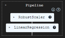
次に、線形回帰モデルをパイプラインにラップしてトレーニングします。

pipe_model = Pipeline([
    ("scaler", RobustScaler()),
    ("LR", LinearRegression())
])

pipe_model.fit(X_train, y_train) # Training a Linear regression model

出力

モデルを評価するために、学習データとテストデータに基づいてターゲットを予測し、その結果をPandasのDataFrameに追加しました。そして、SeabornとMatplotlibを使って予測結果をプロットしました。

# Preparing the data for plotting

train_pred = pipe_model.predict(X_train)
test_pred = pipe_model.predict(X_test)


train_data = pd.DataFrame({
    'Index': range(len(y_train)),
    'True Values': y_train,
    'Predicted Values': train_pred,
    'Set': 'Train'
})

test_data = pd.DataFrame({
    'Index': range(len(y_test)),
    'True Values': y_test,
    'Predicted Values': test_pred,
    'Set': 'Test'
})

# figure size 750x1000 pixels
fig, axes = plt.subplots(2, 1, figsize=(7.5, 10), sharex=False)

# Plot Train Data
sns.lineplot(ax=axes[0], data=train_data, x='Index', y='True Values', label='True Values', color='blue')
sns.lineplot(ax=axes[0], data=train_data, x='Index', y='Predicted Values', label='Predicted Values', color='orange')
axes[0].set_title(f'Train Set: True vs Predicted Values | Acc = {r2_score(y_train, train_pred)}', fontsize=14)
axes[0].set_ylabel('Values', fontsize=12)
axes[0].legend()

# Plot Test Data
sns.lineplot(ax=axes[1], data=test_data, x='Index', y='True Values', label='True Values', color='blue')
sns.lineplot(ax=axes[1], data=test_data, x='Index', y='Predicted Values', label='Predicted Values', color='orange')
axes[1].set_title(f'Test Set: True vs Predicted Values | Acc = {r2_score(y_test, test_pred)}', fontsize=14)
axes[1].set_xlabel('Index', fontsize=12)
axes[1].set_ylabel('Values', fontsize=12)
axes[1].legend()

# Final adjustments
plt.tight_layout()
plt.show()

出力

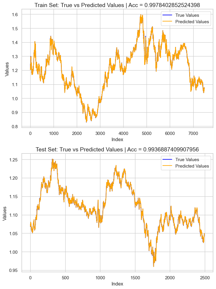
結果として得られたのは、約0.99のR²スコアを持つ過学習したモデルでした。これは、モデルの健全性を示す良い兆候とは言えません。次に、特徴量の重要度を確認し、モデルに好影響を与えている特徴量を観察します。逆に、悪影響を与えている特徴量が検出された場合は、除去していきます。

# Extract the linear regression model from the pipeline
lr_model = pipe_model.named_steps['LR']

# Get feature importance (coefficients)
feature_importance = pd.Series(lr_model.coef_, index=X_train.columns)

# Sort feature importance
feature_importance = feature_importance.sort_values(ascending=False)

print(feature_importance)

出力

macd main            266.706747
close                  0.093652
open                   0.093435
Avg price              0.042505
close lag_1            0.006972
close lag_3            0.003645
bb_upper               0.001423
close lag_5            0.001415
bb_middle              0.000766
high_low               0.000201
bb_lower               0.000087
var close 5 days      -0.000179
ATR 14                -0.000185
close pct_change      -0.001046
close lag_4           -0.002636
close lag_2           -0.003881
open_close            -0.004705
high                  -0.008575
low                   -0.008663
macd histogram     -5504.010453
macd signal        -5518.035201
dtype: float64

最も有益な特徴両はmacd mainでしたが、macd histogramとmacd signalはモデルにとって最も有益な変数ではありませんでした。負の特徴量重要度を持つすべての値を削除し、モデルを再学習させてから、再度精度を確認してみましょう。

X = df.drop(columns=[
    "future_close", # drop the target veriable from the independent variables matrix
    "var close 5 days", 
    "ATR 14", 
    "close pct_change",
    "close lag_4",
    "close lag_2",
    "open_close", 
    "high", 
    "low",
    "macd histogram",
    "macd signal"   
])

pipe_model = Pipeline([
    ("scaler", MinMaxScaler()),
    ("LR", LinearRegression())
])

pipe_model.fit(X_train, y_train)

再学習させたモデルの精度は、以前のモデルと非常に似ており、依然として過学習の状態にありました。現時点ではそれでも問題ありません。次は、モデルをONNX形式でエクスポートする作業に進みましょう。

MQL5での機械学習モデルの展開

エキスパートアドバイザー(EA)内では、まずモデルをリソースとして追加し、プログラムと一緒にコンパイルできるようにします。

ファイル：LR model Test.mq5

#resource "\\Files\\EURUSD.dailytf.model.onnx" as uchar lr_onnx[]

必要なライブラリすべてをインポートします。Pandasライブラリ、ta-lib（インジケーター用）、および線形回帰（モデルの読み込み用）です。

#include <Linear Regression.mqh>
#include <MALE5\pandas.mqh>
#include <ta-lib.mqh>

CLinearRegression lr;

OnInit関数で線形回帰モデルを初期化します。

int OnInit()
  {
//---
   
   if (!lr.Init(lr_onnx))
     return INIT_FAILED;
   
//---
   return(INIT_SUCCEEDED);
  }

この独自のPandasライブラリを使う良い点は、データ収集のコードを一から書き直す必要がないことです。これまで使っていたコードをコピーしてメインのEAに貼り付け、少しだけ修正すれば済みます。

void OnTick()
  {
//---
   
    CDataFrame df;
    int size = 10000; //We collect this amount of bars for training purposes
    
    vector open, high, low, close;
    open.CopyRates(Symbol(), PERIOD_D1, COPY_RATES_OPEN,1, size);
    high.CopyRates(Symbol(), PERIOD_D1, COPY_RATES_HIGH,1, size);
    low.CopyRates(Symbol(), PERIOD_D1, COPY_RATES_LOW,1, size);
    close.CopyRates(Symbol(), PERIOD_D1, COPY_RATES_CLOSE,1, size);
    
    df.Insert("open",open);
    df.Insert("high",high);
    df.Insert("low",low);
    df.Insert("close",close);
    
    
    int lags = 5;
    for (int i=1; i<=lags; i++)
      {
         vector lag = df.Shift("close", i);
         df.Insert("close lag_"+string(i), lag);
      }
    
    vector pct_change = df.Pct_change("close");
    df.Insert("close pct_change", pct_change);
    
    vector var_5 = df.Rolling("close", 5).Var();
    df.Insert("var close 5 days", var_5);
    
    df.Insert("open_close",open-close);
    df.Insert("high_low",high-low);
    
    df.Insert("Avg price",(open+high+low+close)/4);

//---
       
    BB_res_struct bb = CTrendIndicators::BollingerBands(close,20,0,2.000000); //Calculating the bollinger band indicator
    
    df.Insert("bb_lower",bb.lower_band); //Inserting lower band values
    df.Insert("bb_middle",bb.middle_band); //Inserting the middle band values
    df.Insert("bb_upper",bb.upper_band); //Inserting the upper band values
    
    vector atr = COscillatorIndicators::ATR(high,low,close,14);  //Calculating the ATR Indicator
    
    df.Insert("ATR 14",atr); //Inserting the ATR indicator values
    
    MACD_res_struct macd = COscillatorIndicators::MACD(close,12,26,9); //MACD indicator applied to the closing price
    
    df.Insert("macd histogram", macd.histogram); //Inserting the MAC historgram values
    df.Insert("macd main", macd.main); //Inserting the macd main line values 
    df.Insert("macd signal", macd.signal);  //Inserting the macd signal line values 
    
    df.Info();
    CDataFrame new_df = df.Dropnan();
         
    new_df.Head();
    
    string csv_name = Symbol()+".dailytf.data.csv";
    new_df.ToCSV(csv_name, false, 8);
  }

修正点は以下の通りです。

取得するデータ量の変更：以前は1万本のバーを取得していましたが、MACDの期間が26、ボリンジャーバンドが20、ATRが14であるため、約30本あれば十分です。30に設定することで計算に必要な余裕も確保できます。

OnTick関数は非常に頻繁かつ高速に呼び出されるため、新しいティックごとに変数を毎回再定義する必要はありません。

データをCSVファイルに保存する必要はなく、DataFrameの最後の行だけをベクトルに代入してモデルに渡せば十分です。

これらのコードを独立した関数にまとめることで、扱いやすくします。

vector GetData(int start_bar=1, int size=30)
 {
    open_.CopyRates(Symbol(), PERIOD_D1, COPY_RATES_OPEN,start_bar, size);
    high_.CopyRates(Symbol(), PERIOD_D1, COPY_RATES_HIGH,start_bar, size);
    low_.CopyRates(Symbol(), PERIOD_D1, COPY_RATES_LOW,start_bar, size);
    close_.CopyRates(Symbol(), PERIOD_D1, COPY_RATES_CLOSE,start_bar, size);
    
    df_.Insert("open",open_);
    df_.Insert("high",high_);
    df_.Insert("low",low_);
    df_.Insert("close",close_);
    
    
    int lags = 5;
    vector lag = {};
    
    for (int i=1; i<=lags; i++)
      {
         lag = df_.Shift("close", i);
         df_.Insert("close lag_"+string(i), lag);
      }
    
    pct_change = df_.Pct_change("close");
    df_.Insert("close pct_change", pct_change);
    
    var_5 = df_.Rolling("close", 5).Var();
    df_.Insert("var close 5 days", var_5);
    
    df_.Insert("open_close",open_-close_);
    df_.Insert("high_low",high_-low_);
    
    df_.Insert("Avg price",(open_+high_+low_+close_)/4);

//---
       
    BB_res_struct bb = CTrendIndicators::BollingerBands(close_,20,0,2.000000); //Calculating the bollinger band indicator
    
    df_.Insert("bb_lower",bb.lower_band); //Inserting lower band values
    df_.Insert("bb_middle",bb.middle_band); //Inserting the middle band values
    df_.Insert("bb_upper",bb.upper_band); //Inserting the upper band values
    
    atr = COscillatorIndicators::ATR(high_,low_,close_,14);  //Calculating the ATR Indicator
    
    df_.Insert("ATR 14",atr); //Inserting the ATR indicator values
    
    MACD_res_struct macd = COscillatorIndicators::MACD(close_,12,26,9); //MACD indicator applied to the closing price
    
    df_.Insert("macd histogram", macd.histogram); //Inserting the MAC historgram values
    df_.Insert("macd main", macd.main); //Inserting the macd main line values 
    df_.Insert("macd signal", macd.signal);  //Inserting the macd signal line values 
    
       
    CDataFrame new_df = df_.Dropnan(); //Drop NaN values     
    return new_df.Loc(-1); //return the latest row
 }

これが最初に学習用のデータを収集した方法です。この関数内で使われていた特徴量のうち、さまざまな理由で最終モデルには使われなかったものもあり、それらはPythonスクリプト内で削除したのと同様に除外しました。

vector GetData(int start_bar=1, int size=30)
 {
    open_.CopyRates(Symbol(), PERIOD_D1, COPY_RATES_OPEN,start_bar, size);
    high_.CopyRates(Symbol(), PERIOD_D1, COPY_RATES_HIGH,start_bar, size);
    low_.CopyRates(Symbol(), PERIOD_D1, COPY_RATES_LOW,start_bar, size);
    close_.CopyRates(Symbol(), PERIOD_D1, COPY_RATES_CLOSE,start_bar, size);
    
    df_.Insert("open",open_);
    df_.Insert("high",high_);
    df_.Insert("low",low_);
    df_.Insert("close",close_);
    
    
    int lags = 5;
    vector lag = {};
    
    for (int i=1; i<=lags; i++)
      {
         lag = df_.Shift("close", i);
         df_.Insert("close lag_"+string(i), lag);
      }
    
    pct_change = df_.Pct_change("close");
    df_.Insert("close pct_change", pct_change);
    
    var_5 = df_.Rolling("close", 5).Var();
    df_.Insert("var close 5 days", var_5);
    
    df_.Insert("open_close",open_-close_);
    df_.Insert("high_low",high_-low_);
    
    df_.Insert("Avg price",(open_+high_+low_+close_)/4);

//---
       
    BB_res_struct bb = CTrendIndicators::BollingerBands(close_,20,0,2.000000); //Calculating the bollinger band indicator
    
    df_.Insert("bb_lower",bb.lower_band); //Inserting lower band values
    df_.Insert("bb_middle",bb.middle_band); //Inserting the middle band values
    df_.Insert("bb_upper",bb.upper_band); //Inserting the upper band values
    
    atr = COscillatorIndicators::ATR(high_,low_,close_,14);  //Calculating the ATR Indicator
    
    df_.Insert("ATR 14",atr); //Inserting the ATR indicator values
    
    MACD_res_struct macd = COscillatorIndicators::MACD(close_,12,26,9); //MACD indicator applied to the closing price
    
    df_.Insert("macd histogram", macd.histogram); //Inserting the MAC historgram values
    df_.Insert("macd main", macd.main); //Inserting the macd main line values 
    df_.Insert("macd signal", macd.signal);  //Inserting the macd signal line values 
    
    
    df_ = df_.Drop(
       //"future_close", 
       "var close 5 days,"+
       "ATR 14,"+
       "close pct_change,"+
       "close lag_4,"+
       "close lag_2,"+
       "open_close,"+
       "high,"+
       "low,"+
       "macd histogram,"+
       "macd signal"   
    );
    
    CDataFrame new_df = df_.Dropnan();
        
    return new_df.Loc(-1); //return the latest row
 }

上記の関数のように列を削除する代わりに、そもそもそれらを生成するコードを取り除くのが賢明です。不要な計算を減らすことで、多数の特徴量を計算してすぐに削除する際にプログラムが遅くなるのを防げます。

とはいえ、今回はとりあえずDropメソッドを使い続けます。

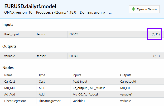
Head()メソッドを呼び出してDataFrameの中身を確認したところ、以下の結果が得られました。

PM      0       15:45:36.543    LR model Test (EURUSD,H1)       CDataFrame::Dropnan completed. Rows dropped: 25/30
HI      0       15:45:36.543    LR model Test (EURUSD,H1)       | open           | close          | close lag_1     | close lag_3     | close lag_5     | high_low       | Avg price      | bb_lower       | bb_middle      | bb_upper       | macd main      |
GK      0       15:45:36.543    LR model Test (EURUSD,H1)       | 1.04057000     | 1.04079000     | 1.04057000      | 1.02806000      | 1.03015000      | 0.00575000     | 1.04176750     | 1.02125891     | 1.03177350     | 1.04228809     | 0.00028705     |
QI      0       15:45:36.543    LR model Test (EURUSD,H1)       | 1.04079000     | 1.04159000     | 1.04079000      | 1.04211000      | 1.02696000      | 0.00661000     | 1.04084750     | 1.02081967     | 1.03210400     | 1.04338833     | 0.00085370     |
PL      0       15:45:36.543    LR model Test (EURUSD,H1)       | 1.04158000     | 1.04956000     | 1.04159000      | 1.04057000      | 1.02806000      | 0.01099000     | 1.04611250     | 1.01924805     | 1.03282750     | 1.04640695     | 0.00192371     |
JR      0       15:45:36.543    LR model Test (EURUSD,H1)       | 1.04795000     | 1.04675000     | 1.04956000      | 1.04079000      | 1.04211000      | 0.00204000     | 1.04743000     | 1.01927184     | 1.03382650     | 1.04838116     | 0.00251595     |
CP      0       15:45:36.543    LR model Test (EURUSD,H1)       | 1.04675000     | 1.04370000     | 1.04675000      | 1.04159000      | 1.04057000      | 0.01049000     | 1.04664500     | 1.01938012     | 1.03447300     | 1.04956588     | 0.00270798     |
CH      0       15:45:36.543    LR model Test (EURUSD,H1)       (5x11)

特徴量は11個あり、モデルにも同じ数の特徴量が表示されます。

以下は、最終モデルの予測を取得するメソッドです。

void OnTick()
  {
     vector x = GetData();  
     Comment("Predicted close: ", lr.predict(x));    
  }

すべてのティックでデータ収集やモデル計算をおこなうのは賢明ではありません。チャートの新しいバーの始まりにのみ計算を実行する必要があります。

void OnTick()
  {
     if (isNewBar())
       {
           vector x = GetData();   
           Comment("Predicted close: ", lr.predict(x)); 
       }
  }

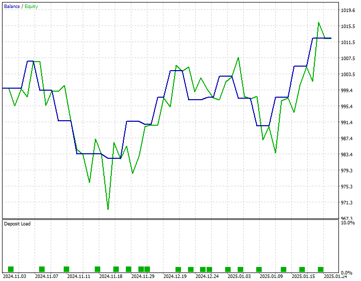
私はシンプルな戦略を開発しました。予測された終値が現在のBidより上回っている場合に買い注文を出し、予測された終値が現在のAskより下回っている場合に売り注文を出すというものです。

以下は、2024年11月1日から2025年1月25日までのストラテジーテスターの結果です。

結論

洗練されたAIモデルをMQL5にインポートし、MetaTrader 5上で簡単に利用できるようになりました。しかし、学習に用いたデータ構造と同様の構造を保持しつつモデルを同期させることは、依然として簡単ではありません。本記事では、PythonのPandasライブラリに馴染みのある機械学習コミュニティやデータサイエンティストの方々にとって扱いやすい環境を目指し、MQL5で2次元データを扱うためのカスタムクラス「CDataFrame」を紹介しました。

MQL5版Pandasライブラリが皆様の開発に役立ち、複雑なAIデータを扱う際の作業を大幅に効率化できることを願っています。

ご一読、誠にありがとうございました。

引き続き、ご注目いただくとともに、以下のGitHubリポジトリにてMQL5言語向け機械学習アルゴリズムの開発にぜひご参加ください。

添付ファイルの表

ファイル名	説明/用途
Experts\LR model Test.mq5	最終的な線形回帰モデルを展開するためのEA
Include\LinearRegression.mqh	ONNX形式で線形回帰モデルを読み込むためのすべてのコードを含むライブラリ
Include\pandas.mqh	DataFrameクラスでデータを操作するためのすべてのカスタムPandasメソッド
Scripts\pandas test.mq5	MLトレーニングの目的でデータを収集するスクリプト
Python\main.ipynb	本稿で使用される線形回帰モデルをトレーニングするためのすべてのコードを含むJupyter Notebookファイル
Files\	ONNXモデルの線形回帰モデルと、AIモデルのトレーニング用のCSVファイルを含むフォルダ

MetaQuotes Ltdにより英語から翻訳されました。
元の記事: https://www.mql5.com/en/articles/17030

添付されたファイル |

ZIPをダウンロード

Attachments.zip (743.15 KB)

警告: これらの資料についてのすべての権利はMetaQuotes Ltd.が保有しています。これらの資料の全部または一部の複製や再プリントは禁じられています。

この著者による他の記事

ディスカッションに移動

MQL5での取引戦略の自動化（第5回）：Adaptive Crossover RSI Trading Suite戦略の開発

この記事では、14期間および50期間の移動平均クロスオーバーをシグナルとして使用し、14期間RSIフィルターで確認するAdaptive Crossover RSI Trading Suiteシステムを開発します。本システムには取引日フィルター、注釈付きのシグナル矢印、監視用のリアルタイムダッシュボードが含まれており、このアプローチにより自動取引の精度と適応性が向上します。

MQL5で自己最適化エキスパートアドバイザーを構築する（第5回）：自己適応型取引ルール

インジケーターを安全に使用する方法を定義したベストプラクティスに従うのは、必ずしも容易ではありません。市場の動きが穏やかな状況では、インジケーターが意図した通りのシグナルを発しないことがあり、その結果、アルゴリズム取引における貴重なチャンスを逃してしまう可能性があります。本稿では、この問題に対する潜在的な解決策として、利用可能な市場データに応じて取引ルールを適応させることが可能な取引アプリケーションの構築方法を提案します。

知っておくべきMQL5ウィザードのテクニック（第53回）：MFI (Market Facilitation Index)

MFI（Market Facilitation Index、マーケットファシリテーションインデックス）は、ビル・ウィリアムズによる指標の一つで、出来高と連動した価格変動の効率性を測定することを目的としています。いつものように、本記事では、ウィザードアセンブリシグナルクラスの枠組みにおいて、このインジケーターのさまざまなパターンを検証し、それに基づいたテストレポートおよび分析結果を紹介します。

プライスアクション分析ツールキットの開発（第10回）：External Flow (II) VWAP

私たちの総合ガイドで、VWAPの力を完全にマスターしましょう。MQL5とPythonを活用して、VWAP分析を取引戦略に統合する方法を学びます。市場に対する洞察を最大限に活かし、より良い取引判断を下せるようになりましょう。