Hilbert-Schmidt Independence Criterion (HSIC)

Introduction

The main task of a trader when working with financial instrument quotes is to create a trading system (EA) with a positive mathematical expectation. When designing such systems, it is often assumed that there are hidden dependencies in the data used for training and subsequent trading. However, the question of statistical testing of this assumption is usually not considered. It is believed that an indirect answer can be obtained through testing results on out-of-sample data.

Meanwhile, a statistically sound answer to the question of whether there is a relationship between the features and the target variable is of key importance. A positive answer supports the use of predictive models, while a negative answer makes one wonder: what exactly is the algorithm trying to predict?

In mathematical statistics, the question of whether a probabilistic dependence exists between random variables is answered by independence tests. One such criterion is the HSIC statistical test, a powerful non-parametric method developed in 2005 by statistician Arthur Gretton.

Unlike the correlation coefficient, which only identifies linear relationships, HSIC is capable of detecting both linear and non-linear relationships. Due to this, it is widely used in machine learning for feature selection, causal analysis, and other tasks. In this article, we will analyze the operating principle of HSIC and implement it in the MQL5 environment.

What is HSIC?

HSIC is a measure of the dependence between two random variables X and Y based on the kernel approach. The method uses the mathematical "magic" of kernel functions (for example, the Gaussian one (Fig. 1)), which transform the data into a special RKHS (Reproducing Kernel Hilbert Spaces) space, where dependencies become easier to detect.

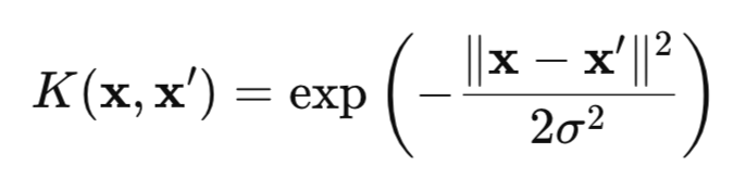
Fig. 1. Gaussian kernel (RBF kernel)

where:

• x, x' – vectors (points) of observations,
• ||   ||² – square of the Euclidean norm,
• σ — kernel width.

There are many kernels that can be used for the HSIC test, such as kernels for categorical data or the Laplace kernel. However, in this article, we will focus our attention on the Gaussian kernel, since it is universal and has the characteristic property. This property allows us to identify any dependencies in the data, making the Gaussian kernel particularly efficient.

Classical HSIC tests pairwise independence between two random variables X and Y by checking whether the condition P(X,Y) = P(X)P(Y) is satisfied. To do this, HSIC analyzes the deviation of the joint distribution from the product of marginal distributions using kernel matrices (a table where each element reflects the similarity between pairs of data points, calculated using a kernel function).

An important advantage of HSIC is its ability to work with data of any dimension: scalar, vector, or combinations of both. This is especially valuable in problems where explicitly constructing multivariate joint distributions P(X,Y) is difficult due to the high dimensionality of the data.

From a mathematical point of view, the HSIC criterion is defined as the square of the Hilbert-Schmidt norm of the cross-covariance operator in RKHS:

where:

• K(X,X') – kernel function for X random variable,
• L(Y,Y') – kernel function for Y random variable,
• ||  ||HS  - Hilbert-Schmidt norm.

Here it is appropriate to compare HSIC with the usual covariance. Classical covariance measures the linear relationship between quantities X and Y in their original space, whereas HSIC works with mappings of X and Y into a reproducing kernel Hilbert space (RKHS), that is, into a space of functions, which allows transforming the data to reveal complex non-linear dependencies.

In practice, the calculation of the Hilbert-Schmidt norm is not required directly. Instead, HSIC is estimated through empirical statistics that rely on kernel matrices constructed for data sample:

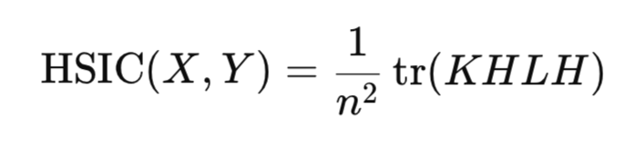
where:

• K,L – n*n kernel matrices,
• H – n*n centering matrix (I -1/n11^T),
• tr() – matrix trace,
• n – number of observations.

Similar to the correlation coefficient, HSIC estimates the presence of a relationship between random variables X and Y using sample statistics, without the need to construct distributions of these variables.

The HSIC statistic is always non-negative:

• HSIC > 0 indicates the presence of dependence,
• whereas HSIC = 0 indicates independence of the data.

HSIC significance test

However, calculating statistics is not sufficient for drawing reliable conclusions. Its statistical significance should be confirmed to exclude a random result. For the HSIC statistic, there is no exact analytical form of the distribution under the null hypothesis. That is, we cannot simply use, for example, a normal distribution and quickly and easily obtain a critical value or p-value without computational costs. There are two main approaches to solving this problem:

• permutation test,
• gamma approximation.

The permutation test is the basic and most accurate method for estimating the HSIC distribution under H0. Its goal is to break any dependence between X and Y by randomly permuting the indices of one of the variables or by shuffling the resulting kernel matrix of that variable. To obtain an accurate result, quite a few such permutations (around 1000) should be performed. Therefore, the permutation test is quite expensive, since it requires computing the HSIC for each such permutation.

The main advantage of the permutation test is that it does not require any assumption about the shape of the data distribution. Instead, it relies on the empirical distribution of the statistic obtained through permutations. The empirical HSIC distribution is then used to obtain a p-value estimate. 

Gamma approximation is used to speed up statistical calculations. In this approach, the HSIC statistic is scaled by the sample size (n*HSIC), and the gamma distribution parameters are estimated from the HSIC sample moments (mean and variance). This method is significantly faster than the permutation test, but its accuracy may be lower for small samples. There are other methods for estimating the HSIC distribution under the null hypothesis of independence, but they are complex to implement and rarely used in practice, so they are not discussed in this article.

Implementing HSIC Permutation in MQL5

The permutation test is implemented in the hsic_test function.

//+------------------------------------------------------------------+
//| Permutation test function                                        |
//+------------------------------------------------------------------+
vector hsic_test(matrix &X,matrix &Y,const double alpha,bool Bootstrap = false,int n_permutations=1000)
{
vector ret = vector::Zeros(3);
int n = (int)X.Rows(); 

matrix K =  RBF_kernel(X); // kernel matrix for X
matrix L =  RBF_kernel(Y); // kernel matrix for Y
matrix H = matrix::Eye(n, n) - matrix::Ones(n, n)/n; // Centering matrix
//--------------------------------------

// Kc centered kernel matrix К
   matrix Kc(n, n);
   if(!Kc.GeMM(H, K, 1.0, 0.0)) {
      Print("Error: Failed to calculate Kc = H * K");
      return ret;
   }
   if(!Kc.GeMM(Kc, H, 1.0, 0.0)) {
      Print("Error: Failed to calculate temp = Kc * H");
      return ret;
   }
   Kc = Kc.Transpose();
   double coef = 1/pow(n,2);

// Calculate the observed value of the HSIC statistic
   double  hsic_obs = compute_hsic(L,Kc,coef);
   ret[0]= hsic_obs;

  //------------ Permutation test ----------------------------------------
  if (Bootstrap == true){ 
    vector hsic_perms = vector::Zeros(n_permutations);   
    for ( int i = 0; i<n_permutations; i++)
    {        
        ShuffleMatrix(L); // Shuffle the matrix
        hsic_perms[i] = compute_hsic(L,Kc,coef);
    }
    
    int count = 0;
for(int i = 0; i < n_permutations; i++)
{
   if(hsic_perms[i] >= hsic_obs)
      count++;
}
   // Calculate the p-value
double p_value = (n_permutations > 0) ? (double)count / n_permutations : 0.0;
    ret[1] = p_value; 
  
  // Calculate the critical value
  double hsic_sort[];
  VectortoArray(hsic_perms,hsic_sort);
  ArraySort(hsic_sort);
  double CV = hsic_sort[(int)round((1-alpha)*n_permutations)];
    ret[2] = CV; 
    }
 //----------------------------------------------------------------------------------   
  return ret;  
}

• The function takes two data sets X and Y (these are matrices of size n*d, where n is the number of observations and d is the dimension of the data),

• the 'alpha' parameter sets the significance level (this is a Type I error, that is, the probability of rejecting the null hypothesis when it is actually true),

• Bootstrap parameter (if 'true', perform a permutation test to obtain a p-value, otherwise, only calculate the statistics),

• n_permutations – number of random permutations,

• the function returns a vector containing the observed HSIC value, p_value, and the critical value for the selected 'alpha' level.

The calculation of the Gaussian kernel matrix is performed in the RBF_kernel function.

//+------------------------------------------------------------------+
//| Gaussian kernel                                                  |
//+------------------------------------------------------------------+ 
matrix RBF_kernel(const matrix &X) {
   int n = (int)X.Rows();
   
   // Calculate the distance matrix using the scalar product
   matrix XX(n, n); 
   if(!XX.GeMM(X, X.Transpose(), 1.0, 0.0)) {
      Print("Error: Failed to calculate XX = X * X^T");    
   }
   
 matrix diag(n,1);
 diag.Col(XX.Diag(),0);  // vector of diagonal elements
 //  squares of distances
 matrix D_sq = matrix::Ones(n, 1).MatMul(diag.Transpose()) + diag.MatMul(matrix::Ones(1, n)) - 2*XX;
   
   // Calculate sigma on the first n_sigma rows
   int n_sigma = MathMin(n, 100);
   int num_elements = (n_sigma * (n_sigma - 1)) / 2;
   vector upper_tri(num_elements);
   int idx = 0;
   for(int i = 0; i < n_sigma; i++) {
      for(int j = i + 1; j < n_sigma; j++) {
         upper_tri[idx] = D_sq[i, j]; 
         idx++;
      }
   }
  double sigma = MathSqrt(0.5 * upper_tri.Median());
   
   return MathExp((-1* D_sq) / (2 * sigma*sigma)); 
}

The function calculates the square of the distances between data points, the width of the sigma kernel, and returns the desired n*n kernel matrix.

To efficiently calculate squared distances, a matrix form is used instead of a regular loop:

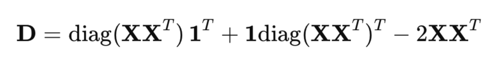
where:

• XX^T - Gram matrix (scalar product matrix),
• diag(XX^T ) - vector of diagonal elements,
• 1 - vector of ones.

The sigma parameter in the Gaussian kernel determines the width of the kernel and significantly affects the sensitivity of HSIC to detecting dependencies in data. The sigma parameter determines the scale of similarity: large sigma values make the kernel wider (points that are further apart are still considered similar), while small values make it narrower (only very close points are considered similar).

One common method for selecting sigma is to use the following median heuristic:

The factor 0.5 is taken to ensure that the RBF kernel denominator is equal to the median of the squared Euclidean distances between data points, which ensures an adaptive estimate that takes into account the scale of the data. 

The n_sigma = MathMin (n, 100) variable limits the amount of data for calculating sigma to 100. This is done to reduce computational costs for large samples while maintaining representativeness for the sigma estimate. The squared Euclidean distances are copied into the upper_tri vector, using only the upper triangle of the distance matrix (excluding the diagonal, i=j) to avoid duplication and zero distances.

Function for calculating HSIC statistics  compute_hsic.

//+------------------------------------------------------------------+
//| Function to calculate HSIC                                       |
//+------------------------------------------------------------------+
double compute_hsic(const matrix &L, const matrix& Kc, const double coef){
matrix KcL= Kc*L;               
return coef*KcL.Sum();
}

After calculating the observed HSIC statistic, a permutation test is performed to test its statistical significance. The ShuffleMatrix(matrix &m) function implements this permutation for the L kernel matrix corresponding to the Y variable. Statistically, it makes no difference whether L or K is shuffled, since HSIC is symmetric with respect to X and Y, giving equivalent results in the permutation test for HSIC. Shuffling the Y variable itself and then recalculating the L matrix for each permutation is inefficient.

//+------------------------------------------------------------------+
//| Function for shuffling matrix data                               |
//+------------------------------------------------------------------+
void ShuffleMatrix(matrix &m)
{
   int rows = (int)m.Rows();
   int cols = (int)m.Cols();
   
   if (rows != cols) {
   Print("Error: Matrix should be square");
}  
   int perm[];
   GeneratePermutation(rows, perm);  // Generate a random permutation of indices
   matrix temp = m;  
   // Rearrange rows and columns
   for(int i = 0; i < rows; i++)
   {
      for(int j = 0; j < cols; j++)
      {
         m[i,j] = temp[perm[i], perm[j]];
      }
   }
}

Generating random indices is done using the GeneratePermutation function.

//+------------------------------------------------------------------+
//| Function to create a random permutation of indices               |
//+------------------------------------------------------------------+ 
void GeneratePermutation(int size, int &perm[])
{
   MathSequence(0,size,1,perm);
   
   // Fisher-Yates algorithm for permutation
   for(int i = size - 1; i > 0; i--)
   {
      // Generate a random index from 0 to i
      int j = (int)(MathRand() / 32768.0 * (i + 1)); 
      int temp = perm[i];
      perm[i] = perm[j];
      perm[j] = temp;
   }
}

After multiple permutations of the L kernel matrix, the empirical distribution of the HSIC statistic under the null hypothesis of independence is formed using the ShuffleMatrix function. The p-value is defined as the proportion of HSIC permutation values that are greater than or equal to the observed statistic. If the p-value is less than the 'alpha' significance level, the null hypothesis of independence is rejected.

The critical value is chosen as the quantile of the empirical distribution at the 1−alpha level, that is, the value above which alpha⋅100% of the HSIC permutation calculations are found.

Implementing HSIC Gamma

The hsic_Gamma_test function is responsible for calculating the Gamma approximation.

//+------------------------------------------------------------------+
//| HSIC Gamma approximation function                                |
//+------------------------------------------------------------------+
double hsic_Gamma_test(matrix &X, matrix &Y, double &CV, double & pvalue)
{
int n = (int)X.Rows(); 

matrix K =  RBF_kernel(X); // kernel matrix for X
matrix L =  RBF_kernel(Y); // kernel matrix for Y
matrix H = matrix::Eye(n, n) - matrix::Ones(n, n)/n; // Centering matrix

   matrix Kc(n, n); // Calculate the centered X kernel matrix  
   if(!Kc.GeMM(H, K, 1.0, 0.0)) {
      Print("Error: Failed to calculate Kc = H * K");
      return 0;
   }
   if(!Kc.GeMM(Kc, H, 1.0, 0.0)) {
      Print("Error: Failed to calculate temp = Kc * H");
      return 0;
   }   
   matrix KcT = Kc.Transpose();
     
   matrix Lc(n, n);  // Calculate the centered Y kernel matrix
   if(!Lc.GeMM(H, L, 1.0, 0.0)) {
      Print("Error: Failed to calculate Lc = H * L");
      return 0;
   }
   
   if(!Lc.GeMM(Lc, H, 1.0, 0.0)) {
      Print("Error: Failed to calculate temp = Lc * H");
      return 0;
      }
              
   double m = (double)n; 
   double coef = 1/m;
   
// Calculate the observed HSIC value
matrix KcLc;
double  hsic_obs = compute_hsic_Gamma(Lc,KcT,coef,KcLc); // n*HSIC

   matrix varHSIC_m = KcLc*KcLc;
   varHSIC_m = (1.0/36.0)*varHSIC_m;  
   double  varHSIC = 1/(m)/(m-1) * (varHSIC_m.Sum() - varHSIC_m.Trace() );
   varHSIC = 72*(m-4)*(m-5)/m/(m-1)/(m-2)/(m-3)  *  varHSIC; // HSIC variance
   
   matrix KD;
   KD.Diag(K.Diag(),0);
   matrix LD;
   LD.Diag(L.Diag(),0);
   K = K-KD;   
   L = L-LD;  
   matrix one = matrix::Ones(n,1);
   matrix a = 1/m/(m-1)*one.Transpose();
   matrix muX;
   muX.GeMM(a,K.MatMul(one),1,0);
   matrix  muY;
   muY.GeMM(a,L.MatMul(one),1,0);
   double mHSIC  = 1/m * ( 1 +muX[0,0]*muY[0,0]  - muX[0,0] - muY[0,0] ) ; // HSIC mathematical expectation

//Gamma distribution parameters
 double alphaG = mHSIC*mHSIC / varHSIC;
 double beta = varHSIC*m / mHSIC;   
 
 int err;
 CV = MathQuantileGamma(1-alpha_,alphaG,beta,err);  // Critical value
 pvalue = 1 - MathCumulativeDistributionGamma(hsic_obs,alphaG,beta,err); // p-value 
 //----------------------------------------------------------------------------------   
  return hsic_obs;  
}

Here we compute the HSIC statistic scaled by the sample size n (n*HSIC), which is approximated by a gamma distribution with shape (alpha) and scale (beta) parameters. These parameters are determined based on the mathematical expectation and variance of the HSIC statistics.

Testing on synthetic data

To evaluate the ability of HSIC to detect non-linear dependencies, we simulate an experiment typical for trading problems. Let's consider two features X={X 1 ,X 2 } that are non-linearly related to the Y scalar target variable, but do not have a linear correlation with it (Fig. 2). This situation reflects a real-world challenge a trader faces: testing whether the selected features influence the predicted variable before using them in a trading system.

Let's generate data as follows:

Y = X1^2 * cos(pi * X2) + Noise

where:

• X1 and X2 - independent and identically distributed uniform variables [-5,5],
• Noise – Gaussian noise,
• Y - target variable, related to X1 and X2 by a non-linear relationship.

Fig. 2. Scatter plot for the Y target variable and X features

The purpose of the experiment is to test the independence hypothesis in the form:

P(X1,X2,Y) = P(X1,X2)P(Y),

that is, to determine whether both features jointly influence the target variable or whether there is no relationship between them.

In real-world problems where the number of features can be large, HSIC allows for flexible testing of dependencies: both for individual features (e.g., X1 or X2 with Y) and for arbitrary subgroups of data. This makes the method useful for selecting informative features, for example, by ranking them by p-value to select the most significant ones for building a trading system.

Figure 3 shows the results of the HSIC test using Gamma approximation. The obtained HSIC value and the corresponding p-value and critical value confirm a statistically significant non-linear relationship between X and Y. This demonstrates the ability of HSIC to effectively identify complex relationships in data, which is particularly important for stock market analysis, where features often have a non-linear effect on the predicted variable. In comparison, the correlation coefficient calculated for X1, X2 and Y turned out to be close to zero, revealing no linear relationship.

Fig. 3. HSIC test results, gamma approximation

The exact HSIC permutation test, run on the same sample size, took 8.5 seconds on the author's rather modest by today's standards PC (a 4-core Ryzen 3). However, the calculation time of the gamma approximation is significantly faster, making it the preferred choice for tasks where computation speed is important, such as when analyzing large volumes of financial data in real time. Gamma approximation, despite possible inaccuracies with small samples, provides a balance between speed and accuracy, making it a valuable tool for implementing HSIC in MQL5 trading algorithms.

Conclusion

In this article, we discussed HSIC (Hilbert-Schmidt Independence Criterion), a powerful non-parametric method for assessing the relationship between random variables. HSIC uses a kernel approach that allows it to identify complex non-linear relationships without the need for explicit modeling of joint distributions.

Key HSIC benefits:

• works with scalar and vector data of any dimension,
• captures complex non-linear dependencies,
• relatively easy to implement

However, the method also has its limitations:

• sensitivity to the choice of the kernel width σ parameter,
• sample size dependence: on small samples, the permutation test may be less powerful, and on large samples, calculating the K and L kernel matrices is quite time-consuming,
• HSIC only indicates the presence of a relationship, but does not characterize its strength, unlike the correlation coefficient.

In this article, we demonstrated the application of HSIC to synthetic data with non-linear dependence, confirming its ability to detect relationships inaccessible to traditional methods, such as Pearson correlation. The implementation of HSIC in MQL5 demonstrated its practical applicability for selecting informative features in the development of trading systems.

We have looked at the basic version of the method with a Gaussian kernel, but HSIC has more advanced capabilities, including handling categorical data and testing conditional independence. These directions open up prospects for further research and application of the method in problems of trading, machine learning, and data analysis.