Econometric tools for forecasting volatility: GARCH model

Introduction

Volatility is an important indicator for assessing the variability of financial asset prices. When analyzing quotes, it has long been noted that large price changes very often lead to even larger changes, especially during financial crises. In turn, small changes are usually followed by small price changes. Thus, calm periods are followed by periods of relative instability.

The first model that attempted to explain this phenomenon was ARCH , developed by Engle — Autoregressive conditional heteroscedasticity (heterogeneity). In addition to the clustering effect (grouping returns into bundles of large and small values), the model also explained the appearance of heavy tails and positive kurtosis, which is characteristic of all distributions of price increments. The success of the ARCH conditional Gaussian model led to the emergence of a number of its generalizations. Their purpose was to provide explanations for a number of other phenomena observed in the analysis of financial time series. Historically, one of the first generalizations of the ARCH model is GARCH (Generalized ARCH) model.

The main advantage of GARCH compared to ARCH lies in the fact it is more parsimonious and does not require a long-lag structure when fitting sample data. In this article, I want to describe the GARCH model and, most importantly, offer a ready-made tool for forecasting volatility based on it since the forecast is one of the main objectives when analyzing financial data.

Non-parametric approach to volatility estimation

Using volatility to assess risks is a fairly popular topic among traders. The most common way to measure volatility is to simply calculate the standard deviation over a given period of time.

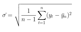
This is the so-called non-parametric approach to volatility estimation. The volatility calculated this way is called historical or empirical volatility. In the Gaussian random walk model, this is the main measure of uncertainty and variability, since it assumes that volatility is constant over time.

Parametric approach to volatility estimation

In the GARCH model, in turn, it is assumed that volatility is a random variable (volatility itself is volatile). This is already closer to reality. The GARCH process is set using the following equations:

where:

• Yt – logarithmic price increments,
• ε t - model residuals
• σt ² - conditional variance
• zt = i.i.d. N(0,1) – standard gaussian distribution
• zt = i.i.d. t-Student(v) – standard Student's t-distribution with v degrees of freedom
• (omega,alpha,beta,v) – model parameters that should be estimated from a data sample

The following restrictions are imposed on the model parameters:

• omega >0, variance positivity condition,
• alpha≥0,
• beta≥0,
• ∑alphai + ∑betaj <1 , stationarity condition,
• v>2

If beta = 0, GARCH model turns into ARCH model.

The GARCH model is usually supplemented by -a model of conditional or unconditional mathematical expectation. For example, the first-order autoregressive process AR(1) can be used as a model of conditional mathematical expectation:

where:

• u – shift parameter,
• A 1 – autoregression model parameter

The goal of conditional mean modeling is to determine a series of squared residuals (εt²) to be used in search for the conditional variance. If there is no auto correlation in the profit series, which is usually the case, then we can move on to the unconditional mathematical expectation model:

In this article, I will use a model without estimating the autocorrelation of profits for simplicity of calculations. Thus, the problem of estimating volatility in the GARCH model is reduced to the parametric problem of finding the model ratios (μ, ω, alpha, beta, v).

Estimating GARCH model parameters using maximum likelihood method

The maximum likelihood method is usually used to find unknown parameters. Assuming a Gaussian distribution of et residuals, the logarithmic likelihood function takes the following form:

If deviations from normality are detected, the standardized Student's t-distribution may be used as an appropriate distribution. For small values of the v (freedom degree) parameter, it demonstrates positive kurtosis and heavier tails than the normal distribution. In this case, the likelihood function takes the following form:

where,

• Г — gamma function
• T – data sample volume

ALGLIB MinBLEIC optimizer

To find the values of the GARCH model parameters, we need to maximize the likelihood function. This requires optimization methods. ALGLIB numerical analysis library can help with this. To maximize the objective function, I chose the MinBLEIC(Bound Linear Equality Inequality Constraints) algorithm.

//+------------------------------------------------------------------+
//|  Objective Function: Gaussian loglikelihood                      |
//+------------------------------------------------------------------+
void CNDimensional_GaussianFunc::Func(CRowDouble &x,double &func,CObject &obj)
  {
//x[0] - mu;
//x[1] - omega;
//x[2] - alpha;
//x[3] - beta;
   double returns[];
   ArrayResize(returns,N1);
   for(int i=0;i<N1;i++)
     {
      returns[i] = MathLog(close[i+1]/close[i]);
     }

   double residuals[];
   ArrayResize(residuals,N1);
   for(int i = 0; i<N1; i++)
     {
      residuals[i] = (returns[i] - x[0]);
     }

   double condVar[];
   ArrayResize(condVar,N1);
   condVar[0] = x[1]/(1-x[2]-x[3]);  // Unconditional Variance

   for(int i=1; i<N1; i++)
     {
      condVar[i] = x[1] + x[2]*MathPow(residuals[i-1],2) + x[3]*condVar[i-1]; // Conditional Variance
     }

   double LLF[],a[],b[];
   ArrayResize(LLF,N1);
   ArrayResize(a,N1);
   ArrayResize(b,N1);
   for(int i=0; i<N1; i++)
     {

      a[i]= 1/sqrt(2*M_PI*condVar[i]);
      if(!MathIsValidNumber(a[i]))
        {
         break;
        }

      b[i]= MathExp(- MathPow(residuals[i],2)/(2 * condVar[i]));
      if(!MathIsValidNumber(b[i]))
        {
         break;
        }

      LLF[i]=MathLog(a[i]*b[i]);
      if(!MathIsValidNumber(LLF[i]))
        {
         break;
        }
     }

   func = -MathSum(LLF); // Loglikelihood
  }

In the GARCH function, which directly addresses the objective function and finds the optimal values of the parameters, it is necessary to:

• specify the initial values of the parameters,
• set the data scale (a very important point the success of optimization depends on),
• specify the boundaries within which parameters may change,
• set linear inequality constraints (we only have one for the alpha + beta <1 stationarity),
• specify the conditions for stopping the optimization algorithm,
• specify the differentiation step.

//+------------------------------------------------------------------+
//|  Function GARCH  Gaussian                                        |
//+------------------------------------------------------------------+
vector GARCH()
  {
   double              x[],s[];
   int                 ct[];
   CMatrixDouble       c;
   CObject Obj;
   CNDimensional_GaussianFunc ffunc;
   CNDimensional_Rep frep;

   double returns[];
   ArrayResize(returns,N1);
   for(int i=0;i<N1;i++)
     {
      returns[i] = MathLog(close[i+1]/close[i]);
     }
   double returns_mean  = MathMean(returns);
   double returns_var = MathVariance(returns);
   double KurtosisReturns = MathKurtosis(returns);
// Print("KurtosisReturns= ",KurtosisReturns);

// Initial parameters ---------------------------
   ArrayResize(x,4);
   x[0]=returns_mean;  //  Mu
   x[1]=returns_var;  // Omega
   x[2]=0.0;         // alpha
   x[3]=0.0;        // beta
//------------------------------------------------------------
   double mu;
   if(NormalizeDouble(returns_mean,10)==0)
     {
      mu = 0.0000001;
     }
   else
      mu = NormalizeDouble(returns_mean,10);
// Set Scale-----------------------------------------------
   ArrayResize(s,4);
   s[0] = NormalizeDouble(returns_mean,10);  //  Mu
   s[1] = NormalizeDouble(returns_var,10); // omega
   s[2] =1;
   s[3] =1;
//---------------------------------------------------------------
// Linearly inequality constrained: --------------------------------
   c.Resize(1,5);
   c.Set(0,0,0);
   c.Set(0,1,0);
   c.Set(0,2,1);
   c.Set(0,3,1);
   c.Set(0,4,0.999); // alpha + beta <= 0.999
   ArrayResize(ct,1);
   ct[0]=-1; // {-1:<=},{+1:>=},{0:=}
//--------------------------------------------------------------
// Box constraints ------------------------------------------------
   double bndl[4];
   double bndu[4];

   bndl[0] = -0.01;  // mu
   bndl[1] = NormalizeDouble(returns_var/20,10);  // omega
   bndl[2] = 0.0;  // alpha
   bndl[3] = 0.0;  // beta

   bndu[0] = 0.01;  // mu
   bndu[1] = NormalizeDouble(returns_var,10);  // omega
   bndu[2] = 0.999;  // alpha
   bndu[3] = 0.999;  // beta
//--------------------------------------------------------------
   CMinBLEICStateShell state;
   CMinBLEICReportShell rep;
   double epsg=0;
   double epsf=0;
   double epsx=0.00001;
   double diffstep=0.0001;
//--- These variables define stopping conditions for the outer iterations:
//--- * epso controls convergence of outer iterations;algorithm will stop
//---   when difference between solutions of subsequent unconstrained problems
//---   will be less than 0.0001
//--- * epsi controls amount of infeasibility allowed in the final solution
   double epso=0.00001;
   double epsi=0.00001;

   CAlglib::MinBLEICCreateF(x,diffstep,state); //---  create optimizer
   CAlglib::MinBLEICSetBC(state,bndl,bndu);  //--- add boundary constraints
   CAlglib::MinBLEICSetLC(state,c,ct);
   CAlglib::MinBLEICSetScale(state,s);
   CAlglib::MinBLEICSetPrecScale(state); // Preconditioner
   CAlglib::MinBLEICSetInnerCond(state,epsg,epsf,epsx);
   CAlglib::MinBLEICSetOuterCond(state,epso,epsi);
   CAlglib::MinBLEICOptimize(state,ffunc,frep,0,Obj);
   CAlglib::MinBLEICResults(state,x,rep);   // Get parameters
//---------------------------------------------------------

   double residuals[],resSquared[],Realised[];
   ArrayResize(residuals,N1);
   for(int i = 0; i<N1; i++)
     {
      residuals[i] = (returns[i] - x[0]);
     }

   MathPow(residuals,2,resSquared);
   ArrayCopy(resSquared_,resSquared,0,0,WHOLE_ARRAY);
   MathSqrt(resSquared,Realised);

   double condVar[],condStDev[];
   double ForecastCondVar,PriceConf_Upper,PriceConf_Lower;
   ArrayResize(condVar,N1);
   condVar[0] = x[1]/(1-x[2]-x[3]);
   for(int i = 1; i<N1; i++)
     {
      condVar[i] = x[1] + x[2]*MathPow(residuals[i-1],2) + x[3]*condVar[i-1];
     }

   double PlotUncondStDev[];
   ArrayResize(PlotUncondStDev,N1);
   ArrayFill(PlotUncondStDev,0,N1,sqrt(condVar[0])); // for Plot
   ArrayCopy(PlotUncondStDev_,PlotUncondStDev,0,0,WHOLE_ARRAY);
   MathSqrt(condVar,condStDev);
// Print("math expectation of conditional standard deviation = "," ",MathMean(condStDev));

   ArrayCopy(Real,Realised,0,0,WHOLE_ARRAY);
   ArrayCopy(GARCH_,condStDev,0,0,WHOLE_ARRAY);

   vector v_Realised, v_condStDev;
   v_Realised.Assign(Realised);
   v_condStDev.Assign(condStDev);
   double MSE=v_condStDev.Loss(v_Realised,LOSS_MSE); // Mean Squared Error
//-----------------------------------------------------------------------------
//-------- Standardize Residuals--------------------------------------
   double z[];
   ArrayResize(z,N1);
   for(int i = 0; i<N1; i++)
     {
      z[i] = residuals[i]/sqrt(condVar[i]);
     }
   ArrayCopy(Z,z,0,0,WHOLE_ARRAY);
//----------------------------------------------------------------------------------

//-------------- JarqueBeraTest for Normality  ----------------------------------
   double pValueJB;
   int JBTestH;
   CAlglib::JarqueBeraTest(z,N1,pValueJB);
   if(pValueJB <0.05)
      JBTestH =1;
   else
      JBTestH=0; // H=0 - data Normal, H=1 data are not Normal
   double Kurtosis = MathKurtosis(z); // Kurosis = 0 for Normal distribution
//---------------------------------------------------------------------------------

//-------------------------------------------------------------------------------------
//-------- Forecast Conditional Variance for m bars
   double FCV[];
   ArrayResize(FCV,forecast_m);
   for(int i = 0; i<forecast_m; i++)
     {
      FCV[i] = sqrt(x[1]*((1-MathPow(x[2]+x[3],i+1))/(1-x[2]-x[3])) + MathPow(x[2]+x[3],i)*(x[2]*MathPow(residuals[N1-1],2) + x[3]*condVar[N1-1])) ;
     }
   ArrayCopy(FCV_,FCV,0,0,WHOLE_ARRAY);
//-----------------------------------------------------------------------------------
   double LLF[];
   double Loglikelihood;
   ArrayResize(LLF,N1);
   for(int i = 0; i<N1; i++)
     {
      LLF[i] = MathLog(1/sqrt(2*M_PI*condVar[i])*MathExp(- MathPow(residuals[i],2)/(2*condVar[i])));
     }
   Loglikelihood = MathSum(LLF);
//--------------------------------------------------------------------------

   ForecastCondVar= x[1] + x[2]*MathPow(residuals[N1-1],2) + x[3]*condVar[N1-1];
   int err1;
   PriceConf_Lower = close[N1]*MathExp(-MathAbs(MathQuantileNormal((1-pci)/2,0,1,err1))*sqrt(x[1] + x[2]*MathPow(residuals[N1-1],2) + x[3]*condVar[N1-1])); // confidence interval pci%
   PriceConf_Upper = close[N1]*MathExp(MathAbs(MathQuantileNormal((1-pci)/2,0,1,err1))*sqrt(x[1] + x[2]*MathPow(residuals[N1-1],2) + x[3]*condVar[N1-1]));  // confidence interval pci%

//--------------------------------------------------------------------------------------
   vector result= {x[0],x[1],x[2],x[3],rep.GetTerminationType(),ForecastCondVar,PriceConf_Lower,PriceConf_Upper,MSE,Loglikelihood,condVar[0],returns_var,JBTestH,Kurtosis};
   return (result);
  }
//+------------------------------------------------------------------+

Volatility forecast using GARCH(1,1) model

Volatility point forecast

Once the model parameters have been found, we can move on to the main task – forecasting volatility. Volatility forecast for the GARCH(1,1) model on m steps forward is calculated using the equation:

where:

• γ = α1 + β 1.

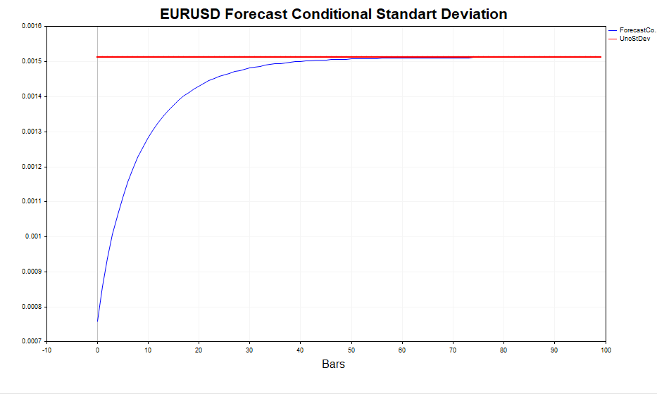
In case of m →∞, the forecast converges to the theoretical unconditional GARCH variance (if the condition of the model stationarity α1+ β1 < 1 is met).

In other words, the more distant the forecast, the closer its values to the stationary value of the unconditional variance. The GARCH script makes it possible to calculate the volatility forecast for m steps forward and compare these values with Eεt ², confirming that this is indeed the case.

Interval forecast

A point forecast of volatility is useful, but it is more important to obtain a probabilistic estimate of the range within which future price increases are to be observed, that is, to obtain confidence intervals with a certain level of significance.

Assuming normality z t= i.i.d. N(0,1) confidence intervals are calculated using the equation:

where:

• q – standard normal distribution quantile

For example, for a confidence interval with a reliability level of 90% (a = 1-0,9), this will be the interval:

[ u – 1,65σ ; u + 1,65σ ]

Things are much more complicated when it is assumed that zt = i.i.d. t-Student(v). In this case, there is no analytical equation for the inverse distribution function. Therefore, to construct confidence intervals, it is necessary to use Monte Carlo simulation.

//+-------------------------------------------------------------------------+
//|Function calculate Forecast Confidence intervals using Monte-Carlo method|
//+-------------------------------------------------------------------------+
bool MCForecastStandardized_t(const double DoF,const double CondStDevForecast,const double prob, double & F_lower[],double & F_upper[])
  {

   double alpha = 1-prob;
   double qlower[1] = {alpha/2};       // q (a/2)
   double qupper[1] = {1-alpha/2};  // q (1-a/2)

   int N = 10000; //number Monte-Carlo simulates
   double h_St[];
   ArrayResize(h_St,N);
   for(int i=0;i<N;i++)
     {
      h_St[i] = CondStDevForecast * Standardized_t(DoF);   // GARCH-Student(1,1)
     }
   MathQuantile(h_St,qlower,F_lower);
   MathQuantile(h_St,qupper,F_upper);
   return(true);
  }

//+--------------------------------------------------------------------------+
//| Function calculate i.i.d. standardized t-distributed variable            |
//+--------------------------------------------------------------------------+
double  Standardized_t(const double DoF)
  {
   double randStandStudent;
   int err;
   randStandStudent = MathRandomNormal(0,1,err) * sqrt(DoF/((MathRandomGamma(DoF/2.0,1)*2.0)));
   randStandStudent = randStandStudent/sqrt(DoF/(DoF-2.0));
   return(randStandStudent);
  }
//+------------------------------------------------------------------+

It is clear that the higher the number of simulations (the default is 10,000), the more accurate the forecast, but the time required for calculations also increases. The most acceptable figure is 100,000. In this case, the confidence intervals look more symmetrical.

Testing the adequacy of the conditionally Gaussian GARCH model

To check the ability of the GARCH model to capture the heteroscedasticity of volatility, it is necessary to check the standardized residuals for autocorrelation and for compliance with the standard normal distribution. Standardized residuals are simply the price increments minus the conditional (or unconditional) mathematical expectation, divided by the conditional standard deviation calculated by the GARCH model.

If the GARCH model is adequate to the actual data, then the standardized residuals will be independent and identically distributed standard normal values.

As an example of residual analysis, let's take daily data on EURUSD over the last four years and calculate the model parameters.

Let's check the squares of the residuals for auto correlation.

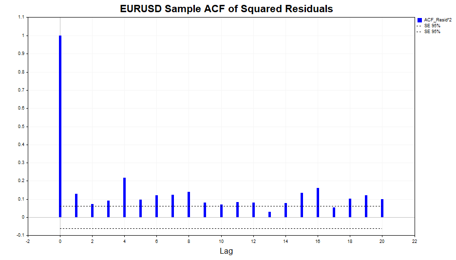
As we can see, there is a slight dependence in the data, up to and including lag 20. Now let's check the squares of the standardized residuals for auto correlation and see if the GARCH(1,1) model was able to adequately describe this dependence.

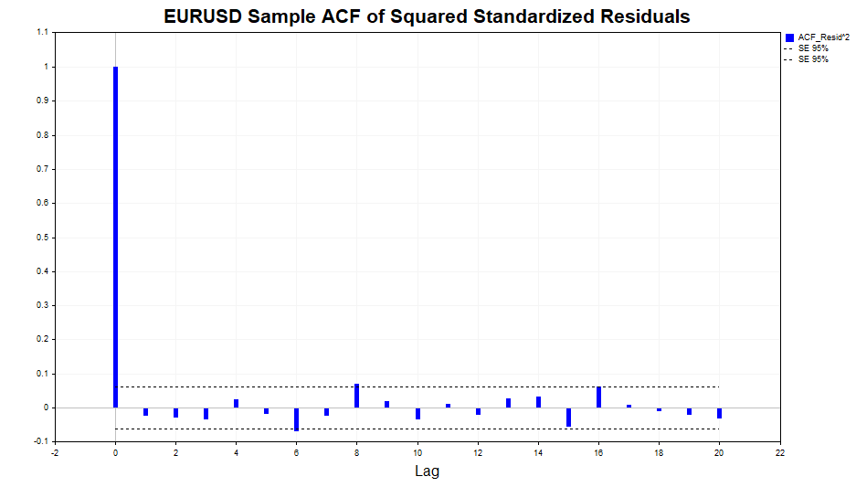
As we can see, the model did a great job. There is no significant correlation in the data.

Let's look at the calculated realized volatility (the square of the logarithmic price increments) and the conditional standard deviation (GARCH). The model responds quite successfully to changes in volatility. The unconditional standard deviation acts as the mean around which the GARCH volatility fluctuates.

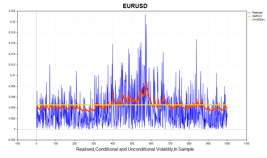
Let's check the normality of the standardized residuals.

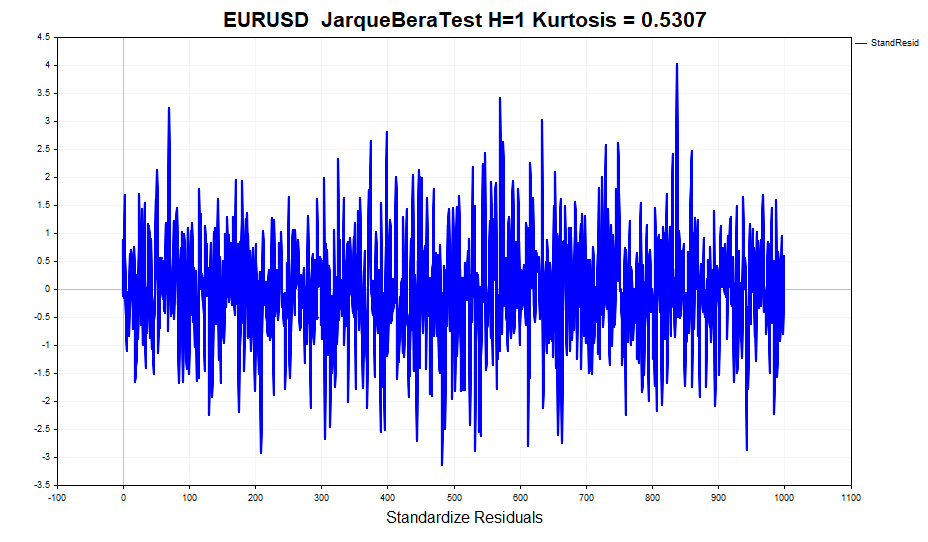
At first glance, the data looks quite normal. There are no clearly visible heavy tails. But formal normality tests, such as the JarqueBeraTest, reject the null hypothesis. The reason lies in the excess (0,5307), which is slightly different from the normal one. At the same time, the excess value for profits is 1.2904. In other words, the GARCH model partially took the effect of peaked distribution into account, although not completely. As you might remember, the unconditional GARCH process distribution has thick tales. This is due to the fact that a mixture of Gaussian distributions with different variances leads to a distribution with heavy tails and positive kurtosis.

Therefore, one of the assumptions of the GARCH model that standardized residuals have a conditional normal distribution is violated. As a consequence, estimates of the model parameters obtained using the maximum likelihood method lose some useful properties, namely, they cease to be asymptotically efficient (in other words, with larger samples, more accurate parameter estimates can be found).

In this case, as an alternative to the normal distribution, we can take the Student's distribution, since with small degrees of freedom it has a positive excess and heavy tails. In this case, the number of degrees of freedom becomes an additional unknown parameter that should be estimated using the sample.

All actions related to the visual display of various statistics that we have just briefly discussed are set in the GARCH script for ease of analysis.

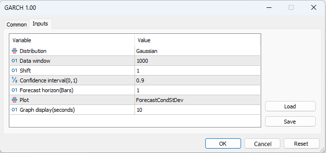
• Distribution – standard normal distribution or standard Student's t-distribution
• Data window - data window for calculating model parameters
• Shift – data window shift (1 - penultimate bar on the chart)
• Confidence interval – confidence interval significance level (the higher the significance level, the wider the confidence interval)
• Forecast horizon – volatility forecast for a given number of bars ahead
• Plot – displays: volatility forecast, standardized residuals, comparison of realized and GARCH volatility, auto correlation function of squared residuals and auto correlation function of standardized squared residuals on the chart.

iGARCH indicator

To get the first idea of the model and the data we want to apply this model to, the GARCH script will do just fine. But to evaluate and forecast volatility in real time, we would like to have an algorithm that will recalculate the model parameters on each new bar, quickly adapting to the constantly changing market. The iGARCH adaptive indicator is the solution to this problem.

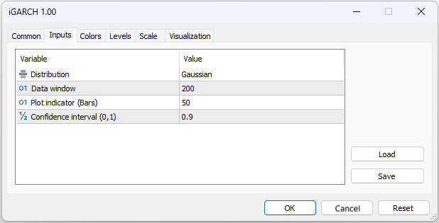
• Plot indicator – number of bars the indicator will be calculated for

The indicator forecasts volatility (conditional standard deviation) and confidence intervals for future price increments with a certain level of one-step-ahead reliability. The forecast is displayed on the zero bar, data for calculating the parameters (Data window) are taken starting from the first bar. Since the model parameters are optimized on each bar, it is not recommended to set too large Plot indicator(Bars) values, since the calculation may take quite a long time (especially for the model with Student's distribution).

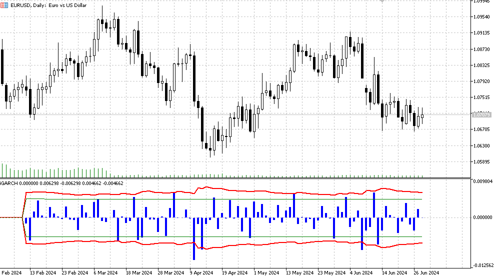
• Histogram - logarithmic profit values LN(Yt/Yt-1),
• The red line is the upper and lower bounds of the conditional standard deviation forecast determined for the confidence interval significance level (default is 90%). This means that in approximately 90% of cases, logarithmic price increments will be within these limits,
• The green lines represent the normal historical volatility, the lower and upper bounds respectively.

Additionally, the following information is displayed in the journal, which is updated at each new bar:

• latest values of optimized parameters (mu, omega, alpha, beta, v),
• likelihood function (LLF) values,
• forecast price levels for the selected significance level,
• report on successful optimization completion,
• values of the predicted conditional standard deviation,
• GARCH theoretical unconditional standard deviation values,
• historical standard deviation values.

Conclusion

I have considered one of the most popular models of conditional heteroscedasticity – the GARCH model. As it has turned out, the standard methods of estimating volatility, which assume its constancy over time, do not reflect the real situation. In contrast, the GARCH model takes into account the variability of volatility over time, which makes it more adequate for analyzing market conditions.

Using the GARCH(1,1) model as an example, an adaptive indicator was developed that allows forecasting volatility and confidence intervals for logarithms of price increases one step ahead in time. This provides the opportunity to obtain a probabilistic assessment of future price changes and thus more effectively manage the risks of open positions.

This indicator allows us to choose not only the classic Gaussian residual model, but also a model that assumes that the residuals follow the Student's distribution. At the same time, optimization of the model parameters is carried out on each new bar, which allows us to quickly respond to the current market situation.

To estimate the model parameters using the maximum likelihood method, we used the MinBLEIC optimization algorithm from the ALGLIB numerical analysis library. The GARCH script calculates all the necessary statistics associated with the model and provides visual tools for assessing dependencies in the data.

Thus, the application of the GARCH model in econometric research and financial analysis allows for more accurate volatility forecasts, which significantly improves risk management and investment decision making.