One-Dimensional Singular Spectrum Analysis

Introduction

Financial markets are characterized by high volatility and complex dynamic processes, which makes forecasting and identifying patterns extremely challenging. Singular spectrum analysis (SSA) is a powerful time series analysis technique that allows the complex structure of a series to be represented as a decomposition into simple components such as trend, seasonal (periodic) variations, and noise. The SSA method, based on linear algebra, does not require stationarity assumptions, making it a universal tool for studying the structure of time series. 

However, the extensive use of vector and matrix algebra theory in the SSA literature creates a fairly high entry barrier, which can make it difficult for unprepared readers to understand the topic and prevent them from grasping all the intricacies and advantages of this method of analysis. The article aims to present the theoretical foundations of SSA in an accessible and clear manner, without which the method becomes a "black box", and also to provide a practical implementation of the described concepts. 

The term SSA should be understood as a whole family of analysis methods, but all of them are based on the sequential application of four steps:

• transformation of a time series into a trajectory matrix (Hankel matrix),
• decomposition of the trajectory matrix into a sum of elementary matrices of rank one,
• grouping of elementary matrices,
• restoration (reconstruction) of a time series.

Let's take a closer look at each of these stages.

Construction of the trajectory matrix

The basic idea is to transform a time series into a matrix that will reflect its structure in multidimensional space. This is done in order to reveal hidden dependencies between successive values of the series. The trajectory matrix is constructed as follows. A one-dimensional sample of a time series of size N is taken and transformed into a set of K vectors (K = N – L + 1) by compiling sliding subsamples of size L (window length). The resulting vectors of length L(x1,x2,...,xL},{x2,x3,...,xL+1}etc. ), are located in columns of the trajectory matrix X.

Fig. 1. X trajectory matrix

Here the L parameter determines the depth of analysis. It is usually set equal to N/2.

Decomposition of the trajectory matrix into a sum of matrices of rank one

After constructing the trajectory matrix, its decomposition is performed. When the singular value decomposition (SVD) of the trajectory matrix serves as such a decomposition, then this analysis method is called basic (Basic-SSA).

Using singular value decomposition, the so-called eigentriples (√λi, Ui, Vi) are constructed, where

• σi = √λi are singular values equal to the root of the eigenvalues of the XX' matrix,
• Ui — left singular vectors,
• Vi — right singular vectors,
• i — number of singular values equal to the rank of the X trajectory matrix.

σi singular values show the weight of each component, with large values corresponding to important patterns (trend, cycles), and small values to noise.

Thus, using the SVD decomposition, the trajectory matrix can be represented as a sum of rank one Xi elementary matrices:

Rank one matrices are the "building blocks" more complex matrices are constructed from.

Let's explain the concept of matrix rank in the context of the SSA method. SSA aims to extract a deterministic signal from a time series. Deterministic sequences, such as an exponential, a polynomial, or a sinusoid, are characterized by finite rank. This is due to the fact that they satisfy linear recurrence relations (LRR), and their trajectory matrices contain a limited number of linearly independent vectors. For example, the trajectory matrix of an exponential sequence has rank 1 (only one linearly independent vector), a sinusoid has rank 2, a polynomial of degree (k) has rank k+1, and so on.

The Rank script demonstrates the concept of rank for deterministic series:

//+------------------------------------------------------------------+
//|                                                         Rank.mq5 |
//|                                                           Eugene |
//|                                             https://www.mql5.com |
//+------------------------------------------------------------------+
#property copyright "Eugene"
#property link      "https://www.mql5.com"
#property version   "1.00"
#property script_show_inputs

input int         N  = 100;                // N - length of generated time series
input int         L  = 30;                 // L - window length
input int         T  = 22;                 // T - period length of sine function
//+------------------------------------------------------------------+
//| Script program start function                                    |
//+------------------------------------------------------------------+
void OnStart()
  {
   matrix X=matrix::Zeros(L,N-L+1);
   vector x_exp= vector::Zeros(N);
   vector x_sinus= vector::Zeros(N);
   vector x_polynom= vector::Zeros(N);
   for(int t=0; t <N; t++)
     {
      x_exp[t] = MathPow(1.01,t);           // 1. Exponential sequence: x_t = 1.01^t
      x_sinus[t] = MathSin(2*M_PI*t/T);     // 2. Sine wave: x_t = sin(2 * pi * t / T)
      x_polynom[t] =  1 + t+ MathPow(t,2);  // 3. Polynomial of degree 2: x_t = 1 + t + t^2
     }
   trajectory_matrix(x_exp,L,X);
   Print("Rank Exponential sequence = ",Rank_SVD(X));
   trajectory_matrix(x_sinus,L,X);
   Print("Rank Sinus sequence = ",Rank_SVD(X));
   trajectory_matrix(x_polynom,L,X);
   Print("Rank Polynom sequence = ",Rank_SVD(X));
  }
//+------------------------------------------------------------------+
//| Trajectory matrix X                                              |
//+------------------------------------------------------------------+
void trajectory_matrix(vector & series,int window_length, matrix & X)
  {
   int N_ = (int)series.Size();
   int L_ = window_length;
   int K = N_ - L_ + 1;
   X=matrix::Zeros(L_,K);
   for(int i=0; i <L_;  i++)
     {
      for(int j=0; j <K;  j++)
        {
         X[i,j] = series[i+j];
        }
     }
  }
//+------------------------------------------------------------------+
//|Finds the rank of a matrix using SVD                              |
//+------------------------------------------------------------------+
int Rank_SVD(matrix & X)
  {
   vector sv;
   matrix U,V;
   double tol = 1e-8;  // Threshold for non-zero values
   X.SingularValueDecompositionDC(SVDZ_N,sv,U,V);
   double threshold = tol * sv.Max();
   int rank=0;
   for(int i=0; i<(int)sv.Size(); i++)
     {
      if(sv[i] > threshold)
         rank++;
     }
   return rank;
  }
//+------------------------------------------------------------------+

Real time series such as stock prices are not finite rank sequences due to the presence of noise, making them full rank series = min(L, K). However, if the series is the sum of a finite-rank deterministic signal and noise, the SSA method is able to approximately extract this signal. Then, prediction is performed only for the deterministic component, and the noise is discarded. To do this, the trajectory matrix (X) is decomposed into elementary matrices of rank 1, from which more complex matrices are then formed that correspond to the useful deterministic signal. This is the key idea of the SSA method.

Grouping

In the grouping step, elementary matrices of rank one are combined into groups, which are interpreted as different components of the series (trend, seasonality, noise). One of the most common ways is to group matrices based on the proximity of the singular values of the X matrix. After m disjoint groups of I are determined, decomposition of the X trajectory matrix can be set as:

For example:

• Itrend = {1} — for a trend,
• Iseasonal = {2,3} — for a seasonality,
• Inoise = {4....,i} — for noise,
  where i = number of singular values.

The graphical representation of left singular vectors is useful for visually assessing the presence of a deterministic signal. For example, if a time series contains a trend, the corresponding singular vector will display a smoothly changing trajectory. In the presence of a periodic component, the pair of singular vectors (since the periodic signal has rank 2) will resemble sinusoids. Singular vectors, visually similar to Gaussian white noise and associated with small singular values, correspond to the noise component. These properties allow grouping of components based on visual analysis of singular vectors.

Restoration (reconstruction) of a time series

The next step is to transform each resulting grouped matrix into a new time series of length N using diagonal averaging:

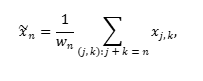
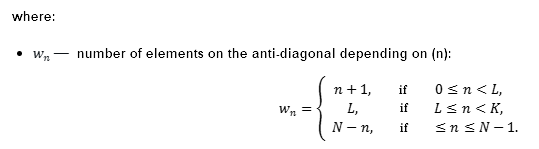
while xj and k are the elements of the grouped (or elementary) matrix.

The time series reconstructed in this way will be responsible either for the trend or for the periodic component. The sum of these series is a non-parametric model of the original time series, which depends on the L window length and the method of grouping the elementary matrices. In this case, the sum of all reconstructed series (including noise) will completely restore the original time series.

Prediction

The forecast of the values of the gi time series for M steps ahead in the SSA method is carried out on the basis of the reconstructed series, using the linear recurrent equation:

where:

• aj  — ratios of LRR (Linear Recurrence Relation)
• fi  — reconstructed series values.

aj ratio vector is determined on the basis of Ui singular vectors:

where:

• First - the first 𝐿 − 1 coordinates of the Ui singular vector,
• Last - the last coordinate of the Ui singular vector,
• 𝑑 — number of selected singular vectors representing the useful signal
  

Toeplitz-SSA

There is another variant of SSA that differs from the traditional approach. Unlike basic SSA, which uses a trajectory matrix based on a sliding window of the time series, Toeplitz-SSA constructs an auto covariance matrix with a Toeplitz structure (hence the name of the method). After which, SVD decomposition is performed for the auto covariance matrix. The grouping method, diagonal averaging, finding LRR ratios and forecasting are performed in exactly the same way as in basic SSA.

Toeplitz-SSA is better suited for analyzing stationary time series (it gives a smaller forecast error compared to the basic one). However, for non-stationary series, classical SSA shows better results. Since we have to deal with non-stationary processes in stock markets, I decided to limit myself to the basic algorithm in this article.

Sample Basic-SSA analysis

Let's move from theory to practical implementation of the described concepts in MQL5 language. For this purpose, a script has been prepared that generates four synthetic time series:

• sine + Gaussian white noise,
• linear trend + sine + Gaussian white noise,
• symmetric Gaussian random walk,
• Gaussian white noise.
  

These series have the following characteristics:

• The first series is stationary, with a periodic component,
• The second one is non-stationary, with a deterministic trend and a periodic component,
• The third one is a non-stationary series with a stochastic trend,
• The fourth one is stationary white noise.
  
  

These models partially cover the spectrum of time series encountered in real-world problems.

The script generates one synthetic series of your choice and sequentially implements the steps we discussed above, and also displays the following graphs on the monitor:

• generated data,
• relative singular values (the proportion of variance of each singular triple),
• the first two singular vectors,
• scatterplot of the first two singular vectors,
• data series + its reconstruction + forecasting,
• reconstruction + forecast using the MQL5SingularSpectrumAnalysisForecast function.
  
  

The graph of relative singular spectral values (the proportion of the square of the singular value from the sum of the squares of all singular values of σi^2/∑ σj^2 — Fig. 2) allows us to determine the type of components that are present in the time series and select the number of singular triplets for signal reconstruction. Typically, components are selected before the point of sharp decline (the so-called "elbow" on the graph).

For a periodic component, there should be two singular values of close magnitude. There may also be a plateau followed by a decline. This means the presence of several harmonic components (sine waves with different frequencies) followed by noise.

A smooth decrease in spectrum values indicates the absence of a deterministic signal.

Fig. 2. Relative spectrum, sinus+noise

It is worth mentioning here the drawback of SSA, which is its inability to distinguish a stochastic trend from a deterministic one. For example, for a random walk series we will have only one pronounced component, which is responsible for the trend. But we all know that this trend is random and unpredictable. To specifically test this case, I included random walk data.

After identifying several of the largest singular values, it is useful to examine the graphs of the corresponding left singular vectors (Fig. 3). For a periodic signal mixed with noise, the first two singular vectors, associated with the largest singular values, usually have a shape close to a sine or cosine wave, reflecting the periodic nature of the signal.

Fig. 3. The first two singular vectors, sinus+noise

Additionally, one can construct a scatter plot for a pair of singular vectors, where the first singular vector (U1) is plotted along the X axis, while the second (U2) one is plotted along the Y axis (Fig. 4).

Fig. 4. Scatterplot of the first two singular vectors, sinus+noise

If the data contains cyclic components, the scatter plot often takes the shape of an ellipse or circle, confirming the sinusoidal nature of the signal. This is because a pair of singular vectors for a periodic component corresponds to two orthogonal harmonics (for example, sine and cosine). If the points in a scatter plot form a chaotic cloud without a clear geometric structure, this indicates the absence of a distinct periodic or deterministic component.

Fig. 5 shows a synthetic sine+noise series, its reconstruction and 100-step-ahead forecast. Visually detecting the presence of a periodic signal in the original data is difficult due to strong noise, but SSA effectively extracts the periodic component. Of course, this is a very simple example, and such a clear picture is rare in real financial data. However, SSA provides an excellent opportunity to confirm or refute the hypothesis of the presence of cycles in prices.

Fig. 5. sinus+noise series forecast

SSA implementation in MQL5

Let's dwell on the existing implementations of SSA in MQL5. The terminal comes with the SingularSpectrumAnalysisForecast function from the Matrix and Vector Methods section\OpenBLAS. From the description of this function, it was not entirely clear to me what kind of SSA it implemented.

Initially, I assumed that this was a variant of Toeplitz-SSA based on the decomposition of the auto covariance matrix. But since the results of the forecast and reconstruction of the series using the Basic-SSA script and the SingularSpectrumAnalysisForecast function completely coincided, then this is probably still an implementation of the basic algorithm. As an example, I will provide a graph of the forecast of the trend+sinus+noise series for three main components (Fig. 6). The analyzed series consists of 200 values, and we make a forecast 100 steps ahead.

Fig. 6. MQL5 vs Basic-SSA reconstruction and forecast series

To decompose the trajectory matrix, I used the SingularValueDecompositionDC function from the same OpenBLAS section, since the developers position the "divide and conquer" algorithm as the fastest among other SVD algorithms. It is very convenient that this function allows us to calculate both full and truncated matrices of singular vectors.

Basic-SSA script code:

//+------------------------------------------------------------------+
//|                                                    Basic-SSA.mq5 |
//|                                                           Eugene |
//|                                             https://www.mql5.com |
//+------------------------------------------------------------------+
#property copyright "Eugene"
#property link      "https://www.mql5.com"
#property version   "1.00"
#property script_show_inputs
#include <Math\Stat\Stat.mqh>
#include <Graphics\Graphic.mqh>

enum SimpleData
  {
   SinusPlusNoise,
   Trend_Sinus_Noise,
   RandomWalk,
   WhiteNoise,
  };

input int         L  = 30;                 // L - window length
input int         N  = 200;                // N - length of generated time series
input int         T  = 22;                 // T - period length of sine function
input int         fs = 100;                // fs - forecast horizon
input int         r_ = 2;                  // r - singular components
input SimpleData  sd = SinusPlusNoise;     // Data
//+------------------------------------------------------------------+
//| Script program start function                                    |
//+------------------------------------------------------------------+
void OnStart()
  {
   int err;
   vector x = vector::Zeros(N); // time series
   double x_array[];
   double original_series[];
//------------1. Data --------------------
//------------------ sinus + noise ---------
   if(sd == SinusPlusNoise)
     {
      for(int i=0; i <N;  i++)
        {
         x[i] = MathSin(2*M_PI*(i+1)/T) + MathRandomNormal(0,1,err);
        }
      VectortoArray(x,x_array);
      ArrayCopy(original_series,x_array,0,0,WHOLE_ARRAY);
      PlotGraphic(x_array,5,1);
     }
//------------------trend + sinus + noise ----
   if(sd == Trend_Sinus_Noise)
     {
      for(int i=0; i <N;  i++)
        {
         x[i] =  0.05 * i + MathSin(2*M_PI*(i+1)/T) + MathRandomNormal(0,1,err);
        }
      VectortoArray(x,x_array);
      ArrayCopy(original_series,x_array,0,0,WHOLE_ARRAY);
      PlotGraphic(x_array,5,1);
     }
//-------------- random walk -----------------
   if(sd == RandomWalk)
     {
      x[0]=100;
      for(int i=1; i <N;  i++)
        {
         x[i] = x[i-1] + MathRandomNormal(0,1,err);
        }
      VectortoArray(x,x_array);
      ArrayCopy(original_series,x_array,0,0,WHOLE_ARRAY);
      PlotGraphic(x_array,5,1);
     }
//-------------- white noise -----------------
   if(sd == WhiteNoise)
     {
      for(int i=0; i <N;  i++)
        {
         x[i] = MathRandomNormal(0,1,err);
        }
      VectortoArray(x,x_array);
      ArrayCopy(original_series,x_array,0,0,WHOLE_ARRAY);
      PlotGraphic(x_array,5,1); // white noise graph
     }
//------------2. Trajectory matrix -------------------
   matrix X;
   trajectory_matrix(x,L,X);
//-------------3. Singular decomposition (SVD) ----
   matrix U, V;
   vector singular_values;
   X.SingularValueDecompositionDC(SVDZ_A,singular_values,U,V);
   V = V.Transpose();
   double total_variance;
   vector powv = singular_values*singular_values;
   total_variance = powv.Sum();
   VectortoArray(powv/total_variance,x_array);
   PlotGraphic(x_array,5,2); // Singular spectrum graph
   double x_1[],x_2[];
   VectortoArray(U.Col(0),x_1);
   VectortoArray(U.Col(1),x_2);
   PlotGraphic(x_1,x_2,5,3); // graph of the first two singular vectors
   PlotGraphic(x_1,x_2,5,4); // scatterplot of the first two singular vectors
//---------- 4. Time series reconstruction----
   int K = N - L + 1;
   matrix X_i = matrix::Zeros(L,K);
   matrix Ui = matrix::Zeros(L,1);
   matrix Vi = matrix::Zeros(1,K);
   vector x_tilde;
   vector recon_series = vector::Zeros(N);
   for(int i=0; i<r_;i++)
     {
      Ui.Col(U.Col(i),0);
      Vi.Row(V.Col(i),0);
      X_i = (Ui.MatMul(Vi))*singular_values[i];  // rank one matrices
      diagonal_averaging(X_i,x_tilde);
      recon_series = recon_series + x_tilde;     // reconstructed series
     }
   double recon[];
   VectortoArray(recon_series,recon);

//------------5. LRR ratio vector   --------------------
   matrix U_r = U;
   U_r.Resize(L,r_);              // r left singular vectors
   vector a = vector::Zeros(L-1); // vector a of LRR ratios
   double denom =0;
   vector u_k;
   double last;
   for(int k=0; k<r_;k++)
     {
      u_k = U_r.Col(k);           //  k th singular vector 

      last = u_k[L-1];
      u_k.Resize(L-1);
      a = a + last*u_k;
      denom = denom + MathPow(last,2);
     }
   denom = 1 - denom;
   a = a/denom;                   // vector a of LRR ratios

//----------------- 6. Forecast using LRR ratios -----------
   int forecast_steps = fs;
   double forecast[];
   ArrayResize(forecast,forecast_steps);
   double fi[];
   ArrayCopy(fi,recon,0,N-L+1,L-1);
   for(int i=0;i<forecast_steps;i++)
     {
      double sum = 0.0;
      for(int j = 0; j < L-1; j++)
        {
         sum += a[j] * fi[j];
        }
      forecast[i]= sum;  // Forecast
      // Update fi
      ArrayCopy(fi, fi, 0, 1, ArraySize(fi)-1); // Shift to the left
      fi[L-2] = forecast[i];                    // Add a new value
     }

   double originalplusforecast[];
   ArrayResize(originalplusforecast,N+forecast_steps);
   ArrayCopy(originalplusforecast,original_series,0,0,WHOLE_ARRAY);
   ArrayCopy(originalplusforecast,forecast,N,0,WHOLE_ARRAY);

   double reconstructedplusforecast[];
   ArrayResize(reconstructedplusforecast,N+forecast_steps);
   ArrayCopy(reconstructedplusforecast,recon,0,0,WHOLE_ARRAY);
   ArrayCopy(reconstructedplusforecast,forecast,N,0,WHOLE_ARRAY);
   PlotGraphic(originalplusforecast,reconstructedplusforecast,15,5);

//---- reconstructed data and forecast using the SingularSpectrumAnalysisForecast function
   vector MQLreconforecast;
   x.SingularSpectrumAnalysisForecast(L,r_,forecast_steps,MQLreconforecast);
   double MQL_RF[];
   VectortoArray(MQLreconforecast,MQL_RF);
   PlotGraphic(reconstructedplusforecast,MQL_RF,10,6);
  }

//+------------------------------------------------------------------+
//| Plot Graphic                                                     |
//+------------------------------------------------------------------+
void PlotGraphic(double &data[], int sec, int n_graph)
  {
   ChartSetInteger(0,CHART_SHOW,false);
   CGraphic graphic;
   ulong width = ChartGetInteger(0,CHART_WIDTH_IN_PIXELS);
   ulong height = ChartGetInteger(0,CHART_HEIGHT_IN_PIXELS);

   if(ObjectFind(0,"Graphic")<0)
      graphic.Create(0,"Graphic",0,0,0,int(width),int(height));
   else
      graphic.Attach(0,"Graphic");

   string st;
   if(sd == SinusPlusNoise)
     {
      st = "Sinus + Noise";
     }
   if(sd == Trend_Sinus_Noise)
     {
      st = "Trend + Sinus + Noise";
     }
   if(sd == RandomWalk)
     {
      st = "Random Walk";
     }
   if(sd == WhiteNoise)
     {
      st = "White Noise ";
     }

   if(n_graph==1) // data graph
     {
      CCurve *curve = graphic.CurveAdd(data,ColorToARGB(clrRed,255),CURVE_LINES,st);
      graphic.XAxis().Name("Series " + st);
      graphic.BackgroundMain(st);
     }
   if(n_graph==2) // chart of singular values (relative_variance = sigma_i^2/Sum Sigma_j^2)
     {
      CCurve *curve = graphic.CurveAdd(data,ColorToARGB(clrBlue,255),CURVE_LINES,st);
      graphic.XAxis().Name("Index ");
      graphic.YAxis().Name("Singular values ");
      graphic.BackgroundMain("Singular values " + st);
     }
   graphic.XAxis().NameSize(18);
   graphic.YAxis().NameSize(18);
   graphic.BackgroundMainColor(ColorToARGB(clrBlack,255));
   graphic.BackgroundMainSize(24);
   graphic.CurvePlotAll();
   graphic.Update();
   Sleep(sec*1000);
   ChartSetInteger(0,CHART_SHOW,true);
   graphic.Destroy();
   ChartRedraw(0);
  }

//+------------------------------------------------------------------+
//| Plot Graphic                                                     |
//+------------------------------------------------------------------+
void PlotGraphic(double &data1[],double &data2[], int sec,int n_graph)
  {
   ChartSetInteger(0,CHART_SHOW,false);
   CGraphic graphic;
   ulong width = ChartGetInteger(0,CHART_WIDTH_IN_PIXELS);
   ulong height = ChartGetInteger(0,CHART_HEIGHT_IN_PIXELS);

   if(ObjectFind(0,"Graphic")<0)
      graphic.Create(0,"Graphic",0,0,0,int(width),int(height));
   else
      graphic.Attach(0,"Graphic");

   if(n_graph==3)
     {
      CCurve *curve =  graphic.CurveAdd(data1,ColorToARGB(clrRed,255),CURVE_LINES,"first");
      CCurve *curve1 = graphic.CurveAdd(data2,ColorToARGB(clrBlue,255),CURVE_LINES,"second");
      graphic.XAxis().Name(" ");
      graphic.BackgroundMain("first and second singular vectors");
     }
   if(n_graph==4) // scatter plot of singular vectors
     {
      CCurve *curve =  graphic.CurveAdd(data1,data2,ColorToARGB(clrRed,255),CURVE_LINES,"first");
      graphic.XAxis().Name("first singular vector");
      graphic.YAxis().Name("second singular vector");
      graphic.BackgroundMain("Scatter plot of singular vectors U_1 vs U_2");
     }

   if(n_graph==5) // data chart plus forecast
     {
      CCurve *curve = graphic.CurveAdd(data1,ColorToARGB(clrBlue,255),CURVE_LINES,"original");
      CCurve *curve1 = graphic.CurveAdd(data2,ColorToARGB(clrRed,255),CURVE_POINTS_AND_LINES,"reconstructed");
      graphic.XAxis().Name("Time ");
      graphic.YAxis().Name("Value ");
      graphic.BackgroundMain("Original(Blue) + reconstructed(Red) + forecast(Red) ");
      curve1.PointsSize(3);
     }

// graph comparing the forecast of the MQL5 SingularSpectrumAnalysisForecast function with the Basic-SSA forecast
   if(n_graph==6)
     {
      CCurve *curve = graphic.CurveAdd(data1,ColorToARGB(clrBlue,255),CURVE_LINES,"BasicSSA");
      CCurve *curve1 = graphic.CurveAdd(data2,ColorToARGB(clrRed,255),CURVE_LINES,"MQL5");
      graphic.XAxis().Name("reconstructed + forecast ");
      graphic.BackgroundMain(" MQL5 SingularSpectrumAnalysisForecast vs script Basic-SSA ");
      curve1.PointsSize(3);
     }
   graphic.XAxis().NameSize(18);
   graphic.YAxis().NameSize(18);
   graphic.BackgroundMainColor(ColorToARGB(clrBlack,255));
   graphic.BackgroundMainSize(24);
   graphic.CurvePlotAll();
   graphic.Update();
   Sleep(sec*1000);
   ChartSetInteger(0,CHART_SHOW,true);
   graphic.Destroy();
   ChartRedraw(0);
  }

//+------------------------------------------------------------------+
//| Copy the vector into an array                                    |
//+------------------------------------------------------------------+
void VectortoArray(vector &v, double &array[])
  {
   int v_size = (int)v.Size();
   ArrayResize(array,v_size);
   for(int i=0; i<v_size; i++)
     {
      array[i]   =  v[i];
     }
  }
//+------------------------------------------------------------------+
//| Trajectory matrix X                                              |
//+------------------------------------------------------------------+
void trajectory_matrix(vector & series,int window_length, matrix & X)
  {
   int N_ = (int)series.Size();
   int L_ = window_length;
   int K = N_ - L_ + 1;
   X=matrix::Zeros(L_,K);
   for(int i=0; i <L_;  i++)
     {
      for(int j=0; j <K;  j++)
        {
         X[i,j] = series[i+j];
        }
     }
  }
//+-------------------------------------------------------------------+
//| Diagonal averaging of a matrix                                    |
//| Input: Xi - matrix L x K (elementary matrix of the i th component)|
//| Output: x_tilde - reconstructed time series                       |
//+-------------------------------------------------------------------+
void diagonal_averaging(matrix &Xi,vector &x_tilde)
  {
   int L_ = (int)Xi.Rows();
   int K  = (int)Xi.Cols();
   int N_ = L_ + K - 1; // Length of the original time series

   x_tilde = vector::Zeros(N_);
   double total; // Sum of elements on the anti diagonal
   int w_n;      // Number of elements on the anti diagonal
   int k;
   for(int n=0; n < N_; n++)
     {
      total = 0;
      w_n = 0;
      for(int j=0; j <L_; j++)
        {
         k = n - j ; // Column index: n = j + k ---> k = n - j
         if(k >= 0 && k < K) // Check that the index is within the matrix
           {
            total = total + Xi[j, k];
            w_n = w_n + 1;
           }
        }
      x_tilde[n] = total / w_n; // Averaging
     }
  }
//+------------------------------------------------------------------+

Conclusion

In this article, we covered the basics of singular spectrum analysis (SSA), a method that uses the singular value decomposition (SVD) of a trajectory matrix to reveal hidden structures in data. We have shown how SSA effectively separates a time series into interpretable components — trend, seasonality, and noise — enabling their reconstruction and forecasting.

However, the method has limitations, in particular the inability to reliably distinguish between deterministic and stochastic trends such as a Gaussian random walk. At the same time, it is worth noting that SSA does not aim to strictly statistically classify trends; its strength lies in its flexible decomposition and identification of data structure, which it copes with successfully.

The application of SSA is not limited to the analysis of univariate time series. The method allows working with multidimensional data. It can be used to construct a change-point detection indicator to detect sudden changes in the behavior of financial instruments. These directions represent promising areas for future research, as a precise understanding of the nature of the data is critical to finding market patterns.